Day 5: Model Selection I Lucas Leemann Essex Summer School - PowerPoint PPT Presentation
Day 5: Model Selection I Lucas Leemann Essex Summer School Introduction to Statistical Learning L. Leemann (Essex Summer School) Day 5 Introduction to SL 1 / 26 1 Motivation 2 Choosing the Optimal Model 3 Subset Selection 4
�� Day 5: Model Selection I Lucas Leemann Essex Summer School Introduction to Statistical Learning L. Leemann (Essex Summer School) Day 5 Introduction to SL 1 / 26
�� 1 Motivation 2 Choosing the Optimal Model 3 Subset Selection 4 Stepwise Selection Forward Stepwise Selection Backwards Stepwise Selection CV vs. Criteria L. Leemann (Essex Summer School) Day 5 Introduction to SL 2 / 26
�� Fundamental Problem: Model Complexity Red: Test error. (Hastie et al, 2008: 220) Blue: Training error. L. Leemann (Essex Summer School) Day 5 Introduction to SL 3 / 26
�� Choosing the Optimal Model • The model containing all of the predictors will always have the smallest RSS and the largest R 2 , since these quantities are related to the training error. • We wish to choose a model with low test error, not a model with low training error. Recall that training error is usually a poor estimate of test error. • Therefore, RSS and R 2 are not suitable for selecting the best model among a collection of models with di ff erent numbers of predictors. L. Leemann (Essex Summer School) Day 5 Introduction to SL 4 / 26
�� Estimating test error: two approaches • We can indirectly estimate test error by making an adjustment to the training error to account for the bias due to overfitting. • We can directly estimate the test error, using either a validation set approach or a cross-validation approach, as discussed in previous lectures. L. Leemann (Essex Summer School) Day 5 Introduction to SL 5 / 26
�� C p , AIC, BIC, and Adjusted R 2 • These techniques adjust the training error for the model size, and can be used to select among a set of models with di ff erent numbers of variables. • The next figure displays C p , BIC, and adjusted R 2 for the best model of each size produced by best subset selection on the Credit data set. L. Leemann (Essex Summer School) Day 5 Introduction to SL 6 / 26
�� Example: Credit data 30000 30000 0.96 0.94 25000 25000 Adjusted R 2 0.92 20000 20000 BIC C p 0.90 15000 15000 0.88 0.86 10000 10000 2 4 6 8 10 2 4 6 8 10 2 4 6 8 10 Number of Predictors Number of Predictors Number of Predictors L. Leemann (Essex Summer School) Day 5 Introduction to SL 7 / 26
�� Mallow’s C p & AIC • Mallow’s C p : C p = 1 ‡ 2 ) , n ( RSS + 2 d ˆ ‡ 2 is an estimate of where d is the total number of parameters used and ˆ the variance of the error ‘ associated with each response measurement. • The AIC criterion is defined for a large class of models fit by maximum likelihood: AIC = 2 logL + 2 ˙ d where L is the maximized value of the likelihood function for the estimated model. • In the case of the linear model with Gaussian errors, maximum likelihood and least squares are the same thing, and C p and AIC are equivalent. L. Leemann (Essex Summer School) Day 5 Introduction to SL 8 / 26
�� Details on BIC BIC = 1 ‡ 2 ) n ( RSS + log ( n ) d ˆ • Like C p , the BIC will tend to take on a small value for a model with a low test error, and so generally we select the model that has the lowest BIC value. ‡ 2 used by C p with a log ( n ) d ˆ ‡ 2 • Notice that BIC replaces the 2 d ˆ term, where n is the number of observations. • Since log ( n ) > 2 for any n > 7, the BIC statistic generally places a heavier penalty on models with many variables, and hence results in the selection of smaller models than C p . L. Leemann (Essex Summer School) Day 5 Introduction to SL 9 / 26
�� Adjusted R 2 • For a least squares model with d variables, the adjusted R 2 statistic is calculated as Adjusted R 2 = 1 − RSS / ( n − d − 1) TSS / ( n − 1) where TSS is the total sum of squares. • Unlike C p , AIC, and BIC, for which a small value indicates a model with a low test error, a large value of adjusted R 2 indicates a model with a small test error. • Maximizing the adjusted R 2 is equivalent to minimizing RSS n − d − 1 . While RSS RSS always decreases as the number of variables in the model increases, n − d − 1 may increase or decrease, due to the presence of d in the denominator. • Unlike the R 2 statistic, the adjusted R 2 statistic pays a price for the inclusion of unnecessary variables in the model. L. Leemann (Essex Summer School) Day 5 Introduction to SL 10 / 26
�� Validation and Cross-Validation • Each of the procedures returns a sequence of models M k indexed by model size k = 0 , 1 , 2 , . . . . Our job here is to select ˆ k . Once selected, we will return model M ˆ k • We compute the validation set error or the cross-validation error for each model M k under consideration, and then select the k for which the resulting estimated test error is smallest. • This procedure has an advantage relative to AIC, BIC, C p , and adjusted R2, in that it provides a direct estimate of the test error. • It can also be used in a wider range of model selection tasks, even in cases where it is hard to pinpoint the model degrees of freedom (e.g. the number of predictors in the model) or hard to estimate the error variance ‡ 2 . L. Leemann (Essex Summer School) Day 5 Introduction to SL 11 / 26
�� Example: Credit data 220 220 220 Cross − Validation Error 200 Square Root of BIC Validation Set Error 200 200 180 180 180 160 160 160 140 140 140 120 120 120 100 100 100 2 4 6 8 10 2 4 6 8 10 2 4 6 8 10 Number of Predictors Number of Predictors Number of Predictors L. Leemann (Essex Summer School) Day 5 Introduction to SL 12 / 26
�� Explaining the example above • The validation errors were calculated by randomly selecting three-quarters of the observations as the training set, and the remainder as the validation set. • The cross-validation errors were computed using k = 10 folds. In this case, the validation and cross-validation methods both result in a six-variable model. • However, all three approaches suggest that the four-, five-, and six-variable models are roughly equivalent in terms of their test errors. • In this setting, we can select a model using the one-standard-error rule. We first calculate the standard error of the estimated test MSE for each model size, and then select the smallest model for which the estimated test error is within one standard error of the lowest point on the curve. L. Leemann (Essex Summer School) Day 5 Introduction to SL 13 / 26
�� Subset Selection L. Leemann (Essex Summer School) Day 5 Introduction to SL 14 / 26
�� Subset Selection: Which Variables? Algorithm: 1 Generate an empty model and call it M 0 2 For each k = 1.... p : " possible models with k explanatory variables ! p i) Generate all k ii) determine the model with the best criteria value (e.g. R 2 ) and call it M k 3 Determine best model within the set of these models: M 0 , ...., M p - rely on CV or a criteria like AIC, BIC, R 2 , or C p L. Leemann (Essex Summer School) Day 5 Introduction to SL 15 / 26
�� Example 1 (1) > regfit.full <- regsubsets(mpg ˜ ., Auto[,-9]) > summary(regfit.full) Subset selection object Call: regsubsets.formula(mpg ˜ ., Auto[, -9]) 7 Variables (and intercept) Forced in Forced out cylinders FALSE FALSE displacement FALSE FALSE horsepower FALSE FALSE weight FALSE FALSE acceleration FALSE FALSE year FALSE FALSE origin FALSE FALSE 1 subsets of each size up to 7 Selection Algorithm: exhaustive cylinders displacement horsepower weight acceleration year origin 1 ( 1 ) " " " " " " "*" " " " " " " 2 ( 1 ) " " " " " " "*" " " "*" " " 3 ( 1 ) " " " " " " "*" " " "*" "*" 4 ( 1 ) " " "*" " " "*" " " "*" "*" 5 ( 1 ) " " "*" "*" "*" " " "*" "*" 6 ( 1 ) "*" "*" "*" "*" " " "*" "*" 7 ( 1 ) "*" "*" "*" "*" "*" "*" "*" L. Leemann (Essex Summer School) Day 5 Introduction to SL 16 / 26
�� Example 1 (2) 0.82 6500 0.78 Adjusted RSq RSS 5500 0.74 4500 0.70 1 2 3 4 5 6 7 1 2 3 4 5 6 7 Number of Variables Number of Variables -450 -500 200 BIC -550 C p 100 -600 50 -650 0 1 2 3 4 5 6 7 1 2 3 4 5 6 7 Number of Variables Number of Variables L. Leemann (Essex Summer School) Day 5 Introduction to SL 17 / 26
�� Subset Selection • Subset selection can be very challenging when p is large since we " possibilities in the k th step. For p = 10 we ! p are then looking at k have about 1000 models and for p = 20 we are already facing more than 1 million models. • What if p >> n ? • Di ff erent approaches: stepwise selection L. Leemann (Essex Summer School) Day 5 Introduction to SL 18 / 26
�� Stepwise Selection L. Leemann (Essex Summer School) Day 5 Introduction to SL 19 / 26
Recommend
More recommend
Explore More Topics
Stay informed with curated content and fresh updates.
