data structures and algorithms 2020 09 28 lecture 9 overview hash - PowerPoint PPT Presentation
data structures and algorithms 2020 09 28 lecture 9 overview hash tables trees dynamic sets elements with key and (possibly) satellite data we wish to add, remove, search (and maybe more) we have seen: heaps, stacks, queues, linked lists
data structures and algorithms 2020 09 28 lecture 9
overview hash tables trees
dynamic sets elements with key and (possibly) satellite data we wish to add, remove, search (and maybe more) we have seen: heaps, stacks, queues, linked lists now: hashing
hashing hash table is an effective data structure for implementing dictionaries keys for example: strings of characters worst-case for operations usually in Θ( n ) with n number of items in practice often much better, search even in O (1) hash table generalizes array where we access address i in O (1) applications of hashing in compilers and cryptography
direct-address table universe of keys: U = { 0 , . . . , m − 1 } with m small use array of length m : T [0 . . . ( m − 1)] what is stored in T [ k ]? either nil if there is no item with key k or a pointer x to the item (or element) with key is x . key = k and possibly satellite data
operations for direct-address table insert( T , x ) add element x T [ x . key ] := x delete( T , x ) remove element x T [ x . key ] := nil search( T , k ) seach for key k return T [ k ] x is pointer to element with key x . key and satelite data x . element
analysis of direct-address table worst-case of inserting, deleting, searching all in O (1) instead of pointer to the object we can store without pointer in the array drawbacks: if universe of keys U is large we need a lot of storage also if we actually use only a small subset of U and: keys must be integers so: hashing
hash tables hash function maps keys to indices (slots) 0 , . . . , m − 1 of a hash table so h : U → { 0 , . . . , m − 1 } element with key k ∈ U hashes to slot h ( k ) usually more keys than indices: | U | >> m space: reduce storage requirement to size of set of actually used keys time: ideally computing a hash value is easy, on average in O (1)
example of a simplistic hash function keys are first names, additional data phone numbers hash function: length modulo 5 (Alice, 0205981555) 0 Alice 1 John 2 (Sue, 0620011223) Sue 3 (John, 0201234567) 4
collisions problem: different keys may be hashed to the same slots namely if h ( k ) = h ( k ′ ) with k � = k ′ this is called a collision if number of keys | U | larger than number of slots m then the hash function h cannot be injective (a function f : A → B is injective if a � = a ′ implies f ( a ) � = f ( a ′ )) even if we cannot totally avoid collisions, we try to avoid as much as possible by taking a ‘good’ hash function
do we often have collisions? for p items and a hash table of size m : m p possibilities for a hash function if p = 8 and m = 10 already 10 8 possibilities m ! there are ( m − p )! possibilities for hashing without collision if p = 8 and m = 10 then 3 · 4 · . . . · 10 such possibilities illustration: birthday paradox for 23 people the probability that everyone has a unique birthday is < 1 2 that is: for p = 23 and m = 366 the probability of collision is ≥ 1 2
how to deal with collisions? either using chaining put items that hash to the same value in a linked list or using open addressing use a probe sequence to find alternative slots if necessary
chaining: example hash function is month of birth modulo 5 drawback: pointer structures are expensive 0 (01.01., Sue) 1 ∅ 2 (12.03., John) (16.08., Madonna) 3 ∅ 4
solving collisions using chaining create a list for each slot link records in the same slot into a list slot in hash table points to head of a linked list and is nil if list is empty
chaining with doubly linked lists: worst-case analysis insert element x in hash table T : in O (1) insert at the front of a doubly linked list delete element x from hash table T : in O (1) if lists are doubly-linked if we have the element available, no search is needed we use the doubly linked structure search key k in hash table T : in O ( n ) with n the size of the dictionary worst-case if every key hashes the same slot, then linear in the total number of elements for exam: know and be able to explain this
load factor assumption: key is hashed to any arbitrary slot, independent of other keys we have n keys and m slots probability of h ( k ) = h ( k ′ ) is 1 m expected length of list at T [ h ( k )] is n m this is called the load factor α = n m
chaining: average case for unsuccessful search: compute h ( k ) and search through the list: in Θ(1 + α ) for successful search: also in Θ(1 + α ) so if α ∈ O (1) (constant!) then average search time in Θ(1) so for example if n ∈ O ( m ) (number of slots proportional to number of keys) if hash table is too small it does not work properly !
intermezzo: choosing a hash function in view of the assumption in the analysis: what is a good hash function? distributes keys uniformly and seemingly randomly regularity of keys distribution should not affect uniformity hash values are easy to compute: in O (1) (these properties can be difficult to check)
possible hash functions with keys natural numbers division method: a key k is hashed to k mod m pro: easy to compute contra: not good for all values of m ; take for m a prime not too close to a power of 2 multiplication method: a key k is hashed to ⌊ ( m · ( k · c − ⌊ k · c ⌋ )) ⌋ with c a constant c with 0 < c < 1 which c is good ? remark: we do not consider universal hashing (book 11.3.3)
open addressing alternative to chaining for solving collisions every slot of the hash table contains either nil or an element for hashing, we make a probe sequence h : U × { 0 , . . . , m − 1 } → { 0 , . . . , m − 1 } that for every key k ∈ U is a permutation of the avalaible slots 0 , . . . , m − 1 we only use the table, no pointers, the load factor is at most 1 for insertion: we try the slots of the probe sequene and take the first available one deletion is difficult, so we omit deletion
remark: removal is difficult suppose the hash function gives probe sequence 2 , 4 , 0 , 3 , 1 for key a , and probe sequence 2 , 3 , 4 , 0 , 1 for key b we insert a , then insert b , then delete a , then search for b if deletion of a gives nil in slot 2, then our search for b fails of deletion of a is marked by a special marker, which is skipped in a search, then search time is also influenced by the amount of markers (not only by the load factor)
open addressing: linear probing next probe: try the next address modulo m h ( k , i ) = h ′ ( k ) + i mod m the probe sequence for a key k is h ′ ( k ) + 0 mod m h ′ ( k ) + 1 mod m h ′ ( k ) + 2 mod m . . . h ′ ( k ) + m − 1 mod m we get clustering! (and removal difficult, as in general for open addressing)
open addressing: double hashing next probe: use the second hash function h ( k , i ) = h 1 ( k ) + i · h 2 ( k ) mod m with h 2 ( k ) relatively prime to the size of the hash table the probe sequence for a key k is: h 1 ( k ) + 0 · h 2 ( k ) mod m h 1 ( k ) + 1 · h 2 ( k ) mod m h 1 ( k ) + 2 · h 2 ( k ) mod m . . . h 1 ( k ) + ( m − 1) · h 2 ( k ) mod m
double hashing: example m = 13, h ( k ) = k mod 13, h ′ ( k ) = 7 − ( k mod 7) h ( k ) h ′ ( k ) try k 18 5 3 5 41 2 1 2 22 9 6 9 44 5 5 5, 10 59 7 4 7 32 6 3 6 31 5 4 5,9,13 73 8 4 8
open addressing: analysis probe sequence: h ( k , 0) , h ( k , 1) , . . . , h ( k , m − 1) assumption: uniform hashing, that is: each key is equally likely to have any one of the m ! permutations as its probe sequence regardless of what happens to the other keys assumption: load factor α = n m < 1
expected number of probes for unsuccessful search probe 1: with probability n m collision, so go to probe 2 probe 2: with probability n − 1 m − 1 collision, so go to probe 3 probe 3: with probability n − 2 m − 2 collision, so go to probe 4 m − i < n n − i note: m = α expected number of probes: m (1 + n − 1 m − 1 (1 + n − 2 1 + n m − 2 ( . . . ))) ≤ 1 + α (1 + α (1 + α ( . . . ))) ≤ 1 + α + α 2 + α 3 + . . . = i =0 α i = Σ ∞ 1 1 − α
open addressing: remarks we assume α < 1 and uniform hashing inserting, and successful or unsuccessful search in O (1) constant then expected number of probes in O (1) if table is full for 50% then we expect 2 probes if table is full for 90% then we expect 10 probes
overview hash tables trees
recap definitions binary tree: every node has at most 2 successors (empty tree is also a binary tree) depth of a node x : length (number of edges) of a path from the root to x height of a node x : length of a maximal path from x to a leaf height of a tree: height of its root number of levels is height plus one
binary tree: linked implementation linked data structure with nodes containing • x . key from a totally ordered set • x . left points to left child of node x • x . right points to right child of node x • x . p points to parent of node x if x . p = nil then x is the root T . root points to the root of the tree (nil if empty tree)
binary tree: alternative implementation remember the heap binary trees can be represented as arrays using the level numbering
tree traversals how can we visit all nodes in a tree exactly once? we will mainly focus on binary trees
Recommend
More recommend
Explore More Topics
Stay informed with curated content and fresh updates.
