Course Objective : to teach you some data structures and associated - PowerPoint PPT Presentation
Course Objective : to teach you some data structures and associated algorithms INF421, Lecture 4 Evaluation : TP not en salle info le 16 septembre, Contrle la fin. Sorting Note: max( CC, 3 4 CC + 1 4 TP ) Organization : fri 26/8, 2/9, 9/9,
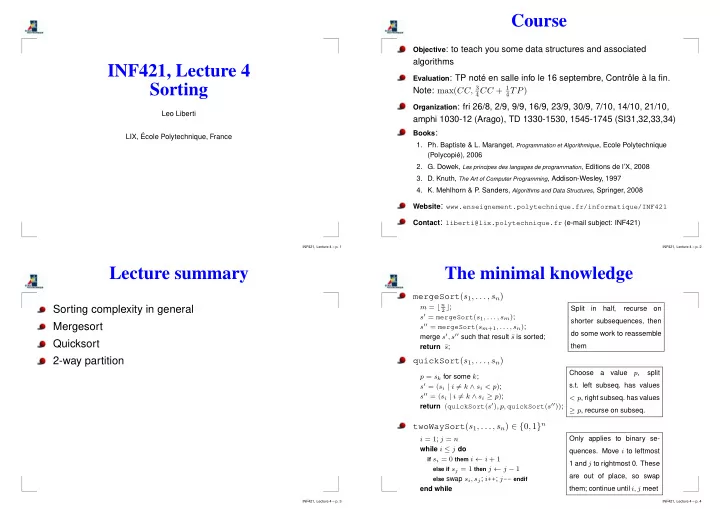
Course Objective : to teach you some data structures and associated algorithms INF421, Lecture 4 Evaluation : TP noté en salle info le 16 septembre, Contrôle à la fin. Sorting Note: max( CC, 3 4 CC + 1 4 TP ) Organization : fri 26/8, 2/9, 9/9, 16/9, 23/9, 30/9, 7/10, 14/10, 21/10, Leo Liberti amphi 1030-12 (Arago), TD 1330-1530, 1545-1745 (SI31,32,33,34) Books : LIX, ´ Ecole Polytechnique, France 1. Ph. Baptiste & L. Maranget, Programmation et Algorithmique , Ecole Polytechnique (Polycopié), 2006 2. G. Dowek, Les principes des langages de programmation , Editions de l’X, 2008 3. D. Knuth, The Art of Computer Programming , Addison-Wesley, 1997 4. K. Mehlhorn & P . Sanders, Algorithms and Data Structures , Springer, 2008 Website : www.enseignement.polytechnique.fr/informatique/INF421 Contact : liberti@lix.polytechnique.fr (e-mail subject: INF421) INF421, Lecture 4 – p. 1 INF421, Lecture 4 – p. 2 Lecture summary The minimal knowledge mergeSort ( s 1 , . . . , s n ) m = ⌊ n 2 ⌋ ; Sorting complexity in general Split in half, recurse on s ′ = mergeSort ( s 1 , . . . , s m ) ; shorter subsequences, then s ′′ = mergeSort ( s m +1 , . . . , s n ) ; Mergesort do some work to reassemble merge s ′ , s ′′ such that result ¯ s is sorted; Quicksort return ¯ s ; them quickSort ( s 1 , . . . , s n ) 2-way partition Choose a value p , split p = s k for some k ; s ′ = ( s i | i � = k ∧ s i < p ) ; s.t. left subseq. has values s ′′ = ( s i | i � = k ∧ s i ≥ p ) ; < p , right subseq. has values return ( quickSort ( s ′ ) , p, quickSort ( s ′′ )) ; ≥ p , recurse on subseq. twoWaySort ( s 1 , . . . , s n ) ∈ { 0 , 1 } n i = 1 ; j = n Only applies to binary se- while i ≤ j do quences. Move i to leftmost if s i = 0 them i ← i + 1 1 and j to rightmost 0. These else if s j = 1 then j ← j − 1 are out of place, so swap else swap s i , s j ; i ++ ; j -- endif end while them; continue until i, j meet INF421, Lecture 4 – p. 3 INF421, Lecture 4 – p. 4
The sorting problem Complexity of a problem? Consider the following problem: Can we ask about the complexity of the sorting problem? S ORTING P ROBLEM (SP). Given a sequence s = ( s 1 , . . . , s n ) , find a permutation π ∈ S n of n symbols Recall: usually the complexity measures the CPU time such that: following property: taken by an algorithm Could ask for the worst-case complexity (over all inputs) ∀ 1 ≤ i < j ≤ n ( s π ( i ) ≤ s π ( j ) ) , of the best algorithm for solving the problem where S n is the symmetric group of order n But how does one list all possible algorithms for a given In other words, we want to order s problem ? The type of s (integers, floats and so on) may be important in order to devise more efficient algorithms: mergeSort and quickSort are for generic types (we assume no This question seems ill-defined prior knowledge); in twoWaySort we know the type is boolean INF421, Lecture 4 – p. 5 INF421, Lecture 4 – p. 6 Comparisons Sorting trees The crucial elements of sorting algorithms are comparisons : given Each sorting tree represents a possible way to chain comparisons as to sort possible inputs s i , s j , we can establish the truth or falsity of the statement s i ≤ s j We can describe any sorting algorithm by means of a sorting tree A sorting tree gives all the possible outputs over all inputs E.g. to order s 1 , s 2 , s 3 , the sorting tree is as follows: Any (comparison-based) sorting algorithm corresponds ? ≤ s 2 s 1 to a particular sorting tree 2 1 The number of (comparison-based) sorting algorithms ? ? is at most the number of sorting trees s 2 ≤ s 3 ≤ s 3 s 2 3 2 2 3 Can use sorting trees to express the idea of best possible sorting algorithm ? ? (13) e s 1 ≤ s 3 s 1 ≤ s 3 3 3 1 1 (23) (132) (12) (123) INF421, Lecture 4 – p. 7 INF421, Lecture 4 – p. 8
Best worst-case complexity The complexity of sorting For any tree T , let | V ( T ) | be the number of nodes of T Let T n be the set of all sorting trees for sequences of length n Tree depth : maximum path length from root to leaf in a tree Different inputs lead to different ordering permutations A binary tree T with depth bounded by k has | V ( T ) | ≤ 2 k in the leaf nodes of each sorting tree ⇒ The sorting tree T ∗ of best algorithm has | V ( T ∗ ) | ≤ 2 B n For a sorting tree T ∈ T n and a π ∈ S n we denote by ℓ ( T, π ) the length of the path in T from the root to the ∀ T ∈ T n , each π ∈ S n appears in a leaf node of T leaf containing π ⇒ Any T ∈ T n has at least n ! leaf nodes, i.e. | V ( T ) | ≥ n ! Best worst-case complexity is, for each n ≥ 0 : Hence, n ! ≤ 2 B n , which implies B n ≥ ⌈ log n ! ⌉ B n = min T ∈ T n max π ∈ S n ℓ ( T, π ) . 1 By Stirling’s approx., log n ! = n log n − ln 2 n + O (log n ) It’s remarkable that we can even formally express such an ⇒ B n is bounded below by a function proportional to n log n apparently ill-defined quantity! (we say B n is Ω( n log n ) ) INF421, Lecture 4 – p. 9 INF421, Lecture 4 – p. 10 Today’s magic result: first part Simple sorting algorithms Complexity of sorting: Ω( n log n ) INF421, Lecture 4 – p. 11 INF421, Lecture 4 – p. 12
Simple sorting algorithms I shall save you the trouble of learning all the numerous types of sorting algorithms in existence Let me just mention selection sort , where you repeatedly Mergesort select the minimum element of s , (3 , 1 , 4 , 2) → (3 , 4 , 2 ) , (1) → ( 3 , 4) , (1 , 2) → ( 4 ) , (1 , 2 , 3) → (1 , 2 , 3 , 4) and insertion sort , where you insert the next element of s in its proper position of the sorted sequence ( 3 , 1 , 4 , 2) → ( 1 , 4 , 2) , (3) → ( 4 , 2) , (1 , 3) → ( 2 ) , (1 , 3 , 4) → (1 , 2 , 3 , 4) Both are O ( n 2 ) ; insertion sort is fast for small | s | INF421, Lecture 4 – p. 13 INF421, Lecture 4 – p. 14 Divide-and-conquer Merge merge ( s ′ , s ′′ ) : merges two sorted sequences s ′ , s ′′ in a Let s = (5 , 3 , 6 , 2 , 1 , 9 , 4 , 3) sorted sequence containing all elements in s ′ , s ′′ Split s midway: the first half is s ′ = (5 , 3 , 6 , 2) and the second is s ′′ = (1 , 9 , 4 , 3) Since s ′ , s ′′ are both already sorted, merging them so that the output is sorted is efficient Sort s ′ , s ′′ : since | s ′ | < | s | and | s ′′ | < | s | we can use Read first (and smallest) elements of s ′ , s ′′ : O (1) recursion; base case is when | s | ≤ 1 (if | s | ≤ 1 then s is Compare these two elements: O (1) already sorted by definition) Get s ′ = (2 , 3 , 5 , 6) and s ′′ = (1 , 3 , 4 , 9) There are | s | elements to process: O ( n ) You can implement this using lists: if s ′ is empty return Merge s ′ , s ′′ into a sorted sequence ¯ s : s ′′ , if s ′′ is empty return s ′ , and otherwise compare the (2 , 3 , 5 , 6) (1 , 3 , 4 , 9) → (1 , 2 , 3 , 3 , 4 , 5 , 6 , 9) = ¯ s first elements of both and choose smallest Return ¯ s INF421, Lecture 4 – p. 15 INF421, Lecture 4 – p. 16
Recursive algorithm Today’s magic result: second part mergeSort ( s ) { 1: if | s | ≤ 1 then return s ; 2: 3: else Complexity of sorting: m = ⌊ | s | 2 ⌋ ; 4: s ′ = mergeSort ( e 1 , . . . , e m ) ; 5: Θ( n log n ) s ′′ = mergeSort ( e m +1 , . . . , e n ) ; 6: return merge ( s ′ , s ′′ ) ; 7: 8: end if } By INF311, mergeSort has worst-case complexity A function is Θ( g ( n )) if it is both O ( g ( n )) and Ω( g ( n )) O ( n log n ) INF421, Lecture 4 – p. 17 INF421, Lecture 4 – p. 18 Divide-and-conquer Let s = (5 , 3 , 6 , 2 , 1 , 9 , 4 , 3) Choose a pivot value p = s 1 = 5 (no particular reason for choosing s 1 ) Partition ( s 2 , . . . , s n ) in s ′ (elements smaller than p ) and Quicksort s ′′ (elements greather than or equal to p ): ( 5 , 3 , 6 , 2 , 1 , 9 , 4 , 3) → (3 , 2 , 1 , 4 , 3) , (6 , 9) Sort s ′ = (3 , 2 , 1 , 4 , 3) and s ′′ = (6 , 9) : since | s ′ | < | s | and | s ′′ | < | s | we can use recursion; base case | s | ≤ 1 Update s to ( s ′ , p, s ′′ ) Notice: in mergeSort , we recurse first , then work on subsequences afterwards . In quickSort , we work on subsequences first , then recurse on them afterwards INF421, Lecture 4 – p. 19 INF421, Lecture 4 – p. 20
Recursive algorithm Partition partition ( s ) : produces two subsequences s ′ , s ′′ of quickSort ( s ) { 1: if | s | ≤ 1 then ( s 2 , . . . , s n ) such that: return ; s ′ = ( s i | i � = 1 ∧ s i < s 1 ) 2: 3: else s ′′ = ( s i | i � = 1 ∧ s i ≥ s 1 ) ( s ′ , s ′′ ) = partition ( s ) ; 4: Scan s : if s i < s 1 put s i in s ′ , otherwise put it in s ′′ quickSort ( s ′ ) ; 5: quickSort ( s ′′ ) ; There are | s | − 1 elements to process: O ( n ) 6: s = ( s ′ , s 1 , s ′′ ) ; 7: You can implement this using arrays; moreover, if you 8: end if use a swap function such that, given i, j , swaps s i with } s j in s , you don’t even need to create any new temporary array: you can update s “in place” INF421, Lecture 4 – p. 21 INF421, Lecture 4 – p. 22 Complexity Worst-case complexity Consider the input ( n, n − 1 , . . . , 1) with pivot s 1 Recursion level 1: p = n , s ′ = ( n − 1 , . . . , 1) , s ′′ = ∅ Worst-case complexity: O ( n 2 ) Recursion level 2: p = n − 1 , s ′ = ( n − 2 , . . . , 1) , s ′′ = ∅ And so on, down to p = 1 (base case) Each partitioning call takes O ( n ) Average-case complexity: O ( n log n ) Get O ( n 2 ) Very fast in practice INF421, Lecture 4 – p. 23 INF421, Lecture 4 – p. 24
Recommend
More recommend
Explore More Topics
Stay informed with curated content and fresh updates.


