Data Cleaning & Checking: Minim ising Garbage Prof. Gavin T L - - PDF document

28/09/2016 1

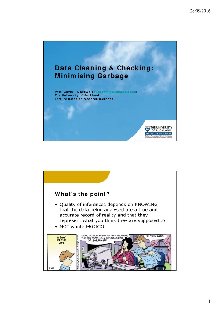
Data Cleaning & Checking: Minim ising Garbage

• Prof. Gavin T L Brow n ( gt.brow n@auckland.ac.nz)

The University of Auckland Lecture notes on research m ethods.

W hat’s the point?

• Quality of inferences depends on KNOWING

that the data being analysed are a true and accurate record of reality and that they represent what you think they are supposed to

• NOT wantedGIGO

28/09/2016 2

• Wrong values
• Response sets
• Jokesters
• Impossible values
• Missing values
• Extreme values

Things that go bum p in the night W rong Values

• Check Sample of Data

Entry cases against SOURCE documents

– 10% systematic sample to start – If all values correct, then proceed – If values wrong, check ALL – Be sure that the digital file represents accurately the source

28/09/2016 3

Response set

• Biased way of responding that invalidates data

– If unwilling, then may be careless/hasty – If unwilling, then may deliberately mislead – If trouble deciding, then may guess or choose socially desirable response

• Look for

– All answers the same—clearly invalid – A physical pattern of responses on the page – Compare logically opposite items; if same answer then maybe responses not valid – Jokesters: Fan, X., Miller, B. C., Park, K.-E., Winward, B. W.,

Christensen, M., Grotevant, H. D., & Tai, R. H. (2006). An Exploratory Study about Inaccuracy and Invalidity in Adolescent Self-Report Surveys. Field Methods 18(3), 223-244. doi: 10.1177/ 152822X06289161

Count Missing responses

• Select range of

items to check— inventory specific.

• Reject cases

with >10% missing

• Mark each case

as to whether it is kept or not

28/09/2016 4

I m possible Values

• Check Minimum & Maximum are valid

– Cannot be higher or lower than allowed

• Check all responses are valid codes

– 0 is not a code, it is a value – Missing response should be obvious arbitrary code (e.g., -9)

• Check logic of inter-linked responses

– e.g., If Year 8, age<14; if school=intermediate, year=7 or 8

• nly; if sex=F, single sex

school≠Male; etc. – Maximum count is 100%

I m agine a strange m issing pattern

Cas e 1 2 3 4 5 6 7 8 9 A . 2 3 4 5 1 2 3 4 B 1 . 3 4 5 1 2 3 4 C 3 4 . 4 5 1 2 3 4 D 3 4 4 . 1 2 3 4 5 E 3 4 4 1 . 1 2 3 4 F 4 5 4 1 5 . 2 4 5 G 3 4 5 1 5 4 . 1 3 H 4 5 4 2 5 4 3 . 2 I 1 2 5 1 1 4 3 2 .

Any analysis that requires all people to answer all items will fail even though each person is missing only 1 answer

28/09/2016 5

Missing Values

• Too much missing

– >10%delete case/variable

• A little missing

– <10% within tolerance – Goal: prevent listwise dropping of otherwise valid cases

Types of m issing data

Source:

Teresa A. Myers (2011). Goodbye, listwise deletion: Presenting Hot Deck Imputation as an easy and effective tool for handling missing data. Communication Methods & Measures, 5(4), 297-310

28/09/2016 6

Expectation Maxim isation

• Impute missing with EM procedure

– EM uses MLE to check that M, SD, correlations, covariances not disturbed by imputation – Assumption is that the sample input values are the best estimate of the population values

• Requires sampling to be high quality

– Iteratively imputes values and checks which values disturb resulting matrices least – PS check descriptives and MCAR test post- imputation to be sure EM variables are ok to use

EM Missing Value Analysis—Setup

28/09/2016 7

MVA: EM

• Check the %

missing per variable.

• IF <10% proceed,
• therwise delete

variable.

Checking MVA effects

• How large a difference did imputation make to

M and SD?

– Usually 2nd & 3rd decimal point

28/09/2016 8

Validity of I m putation

• Distribution of missing should be random
• EM provides Little’s X2 test of Missing

Completely at Random (MCAR)

– Missing value not dependent on any other variable

• When in doubt divide χ2/df and look up the

stat sig of that value. See http://www.fourmilab.ch/rpkp/experiments/an alysis/chiCalc.html χ2/df=1.25; p=.26

Check the im putation for possible invalid im putations

Find the offending case (sort ascending or descending) Correct it to valid min or max value Use these values

28/09/2016 9

I m port im puted values back into m aster data file

• Use data merge procedure but

– Rename variables so that they have slightly different file names. For example

• add an o for original to the original var
• Add an m for missing to the new var

– Put data in ascending order for the key variable

• Unique identifier that you used

Merge variables

• Run Merge <add

variables>

• Match files using key

variable

28/09/2016 10

Extrem e Values

• Do not represent well normal conditions

– Mean is very sensitive to extreme values – Need to detect and resolve (adjust or delete)

• Outlier detection

– Check kurtosis & skewness

• (+/-3.0 no problem)+in some cases as high as 7.00 is
• k

– Check boxplot displays for people with extreme values per variable

Dealing w ith non-norm ality

• Remove
• Robustify (adjust using a trimming technique)

– Use Median or median absolute difference to substitute for Mean and SD if outliers present – Huber’s method or winsorise:

• 90% Winsorised mean sets the bottom 5% to the 5th percentile

value, the top 5% to the 95th percentile value, and then evaluates the variable for normality—repeat until normal.

– http://www.rsc.org/images/brief6_tcm18-25948.pdf

28/09/2016 11

Dealing w ith non-norm ality

• Transform (multiply by a

constant to make normal

• r linear)

– Bulging rule—depending on shape of distribution try these transformations to make variable linear

• Mosteller, Frederick, &

Tukey, John W. (1977). Data Analysis and Regression: A Second Course in Statistics. Reading, MA: Addison- Wesley.

Dealing w ith Non-norm ality

• Square root transformation.

– Add constant so min=2.00

• Log transformation(s).

– Add constant so min=1.00

• Inverse transformation.

– After *-1, add constant so min = 1.00

• Bew are: transformations

improve normality, but curvilinear transformations affect interpretation of results

Osborne, J. W. (2002). Notes on the use of data transformations. Practical Assessment, Research & Evaluation, 8(6), PAREonline.net/getvn.asp?v=8&n=6.

28/09/2016 12

Box-Cox transform ation for non- norm ality

• 1. assess variable to find the optimal power

transformation (λopt).

– Use online software produced by Wessa (2013)

• 2. add/subtract constant (c) to make variable

min = 1.00

• 3. transform each value: (x +/- c)λopt

– Box, G. E. P., & Cox, D. R. (1964). An analysis of transformations. Journal

• f the Royal Statistical Society, B26, 211-234.

– Osborne, J. (2010). Improving your data transformations: Applying the Box-Cox transformation. Practical Assessment, Research & Evaluation, 15(12), http://pareonline.net/pdf/v15n12.pdf. – Wessa, P. (2013). Box-Cox Normality Plot—Free Statistics Software. Office for Research Development and Education, version 1.1.23-r7. Retrieved from http://www.wessa.net/rwasp_boxcoxnorm.wasp

W hen in doubt

• Test the transformation by conducting

Sensitivity analysis

– Run the analysis using the original and transformed values – Evaluate the results for the substantive impact

• Example from Osborne 2010

– correlation between number of faculty (many small universities, few large ones) and associate professor salary (before transformation) r (1161) = 0.49, p < .0001. (% variance accounted for =0.24) – After optimal transformation, r (1161) = 0.66, p < .0001. % variance accounted for = 0.44 (an 81.5% increase) – Which is correct? Make the argument for the better result

28/09/2016 13

Support m aterial

• http://www.tulane.edu/~panda2/Analysis2/datclean/dat

aclean.htm

• http://www.amstat.org/publications/jse/v13n3/datasets

.holcomb.html#Mason

• Robson, C. (2002). Real World Research (2nd ed.) (pp.

391-398). Oxford: Blackwell.

• McClelland, G. H. (2000). Nasty data: Unruly, ill-

mannered observations can ruin your analysis. In H. T. Reis & C. M. Judd (Eds.). Handbook of research methods in social and personality psychology (pp. 393- 411). Cambridge: Cambridge University Press.