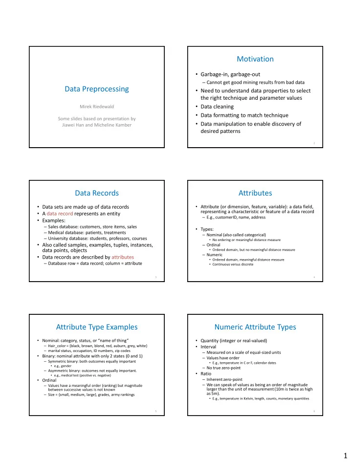
Motivation Garbage-in, garbage-out Cannot get good mining results - PDF document

Motivation • Garbage-in, garbage-out – Cannot get good mining results from bad data Data Preprocessing • Need to understand data properties to select the right technique and parameter values • Data cleaning Mirek Riedewald • Data formatting to match technique Some slides based on presentation by • Data manipulation to enable discovery of Jiawei Han and Micheline Kamber desired patterns 2 Data Records Attributes • Data sets are made up of data records • Attribute (or dimension, feature, variable): a data field, representing a characteristic or feature of a data record • A data record represents an entity – E.g., customerID, name, address • Examples: – Sales database: customers, store items, sales • Types: – Medical database: patients, treatments – Nominal (also called categorical) – University database: students, professors, courses • No ordering or meaningful distance measure • Also called samples, examples, tuples, instances, – Ordinal data points, objects • Ordered domain, but no meaningful distance measure – Numeric • Data records are described by attributes • Ordered domain, meaningful distance measure – Database row = data record; column = attribute • Continuous versus discrete 3 4 Attribute Type Examples Numeric Attribute Types • Nominal: category, status, or “name of thing” • Quantity (integer or real-valued) – Hair_color = {black, brown, blond, red, auburn, grey, white} • Interval – marital status, occupation, ID numbers, zip codes – Measured on a scale of equal-sized units • Binary: nominal attribute with only 2 states (0 and 1) – Values have order – Symmetric binary: both outcomes equally important • E.g., temperature in C or F, calendar dates • e.g., gender – No true zero-point – Asymmetric binary: outcomes not equally important. • Ratio • e.g., medical test (positive vs. negative) – Inherent zero-point • Ordinal – We can speak of values as being an order of magnitude – Values have a meaningful order (ranking) but magnitude larger than the unit of measurement (10m is twice as high between successive values is not known as 5m). – Size = {small, medium, large}, grades, army rankings • E.g., temperature in Kelvin, length, counts, monetary quantities 5 6 1

Discrete vs. Continuous Attributes Data Preprocessing Overview • Discrete Attribute • Descriptive data summarization – Has only a finite or countably infinite set of values • Data cleaning – Nominal, binary, ordinal attributes are usually discrete • Data integration – Integer numeric attributes • Continuous Attribute • Data transformation – Has real numbers as attribute values • Summary • E.g., temperature, height, or weight – Practically, real values can only be measured and represented using a finite number of digits – Typically represented as floating-point variables 7 8 Measuring the Central Tendency Measuring Data Dispersion: Boxplot n 1  • Sample mean: •  Quartiles: Q 1 (25th percentile), Q 3 (75th percentile) x x i – Inter-quartile range: IQR = Q 3 – Q 1 n n   i 1 w x – Various definitions for determining percentiles, e.g., for N records, the p-th i i • Weighted arithmetic mean:   percentile is the record at position (p/100)N+0.5 in increasing order i 1 x – If not integer, round to nearest integer or compute weighted average n  w – E.g., for N=30, p=25 (to get Q1): 25/100*30+0.5 = 8, i.e., Q1 is 8-th largest of the 30 i values  1 i – E.g., for N=32, p=25: 25/100*32+0.5 = 8.5, i.e., Q1 is average of 8-th and 9-th largest – Trimmed mean: set weights of extreme values to zero values • Boxplot: ends of the box are the quartiles, median is marked, whiskers • Median extend to min/max – Middle value if odd number of values; average of the middle – Often plots outliers individually two values otherwise – Outlier: usually, a value higher (or lower) than 1.5 x IQR from Q3 (or Q1) • Mode – Value that occurs most frequently in the data – Unimodal, bimodal, trimodal distribution 9 10 Histogram Measuring Data Dispersion: Variance • Graph display of • Sample variance (aka second central tabulated frequencies, shown as bars moment): n n • 1  1  Shows what proportion      2 2 2 2 m s ( x x ) x x of cases fall into each 2 n i i n n   category i 1 i 1 • Standard deviation = square root of variance • Area of the bar denotes the value, not • Estimator of true population variance from a the height – Crucial distinction sample: n when the categories 1    2 2 s ( x x ) are not of uniform  1  n i n 1 width!  i 1 11 12 2

Scatter plot Correlated Data • Visualizes relationship between two attributes, even a third (if categorical) – For each data record, plot selected attribute pair in the plane 13 14 Not Correlated Data Data Preprocessing Overview • Descriptive data summarization • Data cleaning • Data integration • Data transformation • Summary 15 16 Why Data Cleaning? Example: Bird Observation Data • Data in the real world is dirty • Change of range boundaries over time, e.g., for temperature • Different units, e.g., meters versus feet for elevation – Incomplete: lacking attribute values, lacking certain • Addition or removal of attributes over the years attributes of interest, or containing only aggregate • Missing entries, especially for habitat and weather data – People want to watch birds, not fill out long forms • GIS data based on 30m cells or 1km cells • E.g., occupation=“ ” • Location accuracy – Noisy: containing errors or outliers – ZIP code versus GPS coordinates – Walk along transect but report only single location • E.g., Salary=“ - 10” • Inconsistent encoding of missing entries Hairy vs. Downy Woodpecker – Inconsistent: containing discrepancies in codes or – 0, -9999, -3.4E+38 — need context to decide • Varying observer experience and capabilities names – Confusion of species • E.g., Age=“42” and Birthday=“03/07/1967” – Missed species that was present • E.g., was rating “1, 2, 3”, now rating “A, B, C” • Confusion about reporting protocol – Report max versus sum seen • E.g., discrepancy between duplicate records – Report only interesting species, not all 17 18 3

How to Handle Missing Data? How to Handle Noisy Data? • Ignore the record • Noise = random error or variance in a measured variable – Usually done when class label is missing (for classification tasks) • Typical approach: smoothing • Fill in manually • Adjust values of a record by taking values of other “nearby” – Tedious and often not clear what value to fill in records into account • Dozens of approaches • Fill in automatically with one of the following: • Binning, average over neighborhood – Global constant, e.g., “unknown” • Regression: replace original records with records drawn from • “Unknown” could be mistaken as new concept by data mining regression function algorithm • Identify and remove outliers, possibly involving human inspection – Attribute mean – Attribute mean for all records belonging to the same class • For this class: don’t do it unless you understand the nature – Most probable value: inference-based such as Bayesian formula of the noise or decision tree • A good data mining technique should be able to deal with noise • Some methods, e.g., trees, can do this implicitly in the data 19 20 Data Preprocessing Overview Data Integration • Combines data from multiple sources into a coherent store • Descriptive data summarization • Entity identification problem • Data cleaning – Identify real world entities from multiple data sources, e.g., Bill Clinton = William Clinton • Data integration • Detecting and resolving data value conflicts – For the same real world entity, attribute values from different • Data transformation sources might be different – Possible reasons: different representations, different scales, e.g., • Summary metric vs. US units • Schema integration: e.g., A.cust-id  B.cust-# – Integrate metadata from different sources – Can identify identical or similar attributes through correlation analysis 23 24 Covariance (Numerical Data) Covariance Example • Covariance computed for data samples • Suppose two stocks A and B have the (A 1 , A 2 ,..., A n ) and (B 1 , B 2 ,..., B n ): following values in one week: 1 n 1 n         – A: (2, 3, 5, 4, 6) Cov( A , B ) ( A A )( B B ) A B A B i i i i n n   i 1 i 1 – B: (5, 8, 10, 11, 14) • – AVG(A) = (2 + 3 + 5 + 4 + 6)/ 5 = 20/5 = 4 If A and B are independent, then Cov(A, B) = 0, but the converse is not true – AVG(B) = (5 + 8 + 10 + 11 + 14) /5 = 48/5 = 9.6 – Two random variables may have covariance of 0, but are not independent – Cov(A,B) = (2  5+3  8+5  10+4  11+6  14)/5 − 4  9.6 = 4 • If Cov(A, B) > 0, then A and B tend to rise and fall together • Cov(A,B) > 0, therefore A and B tend to rise – The greater, the more so • If covariance is negative, then A tends to rise as B falls and vice and fall together versa 25 26 4