cvcrand and cptest : Efficient Design and Analysis of Cluster - PowerPoint PPT Presentation
cvcrand and cptest : Efficient Design and Analysis of Cluster Randomized Trials John Gallis in collaboration with Fan Li, Hengshi Yu and Elizabeth L. Turner Duke University Department of Biostatistics & Bioinformatics and Duke Global Health
cvcrand and cptest : Efficient Design and Analysis of Cluster Randomized Trials John Gallis in collaboration with Fan Li, Hengshi Yu and Elizabeth L. Turner Duke University Department of Biostatistics & Bioinformatics and Duke Global Health Institute July 28, 2017 John Gallis cvcrand : Efficient Design and Analysis of CRTs 1 / 34
Presentation Outline 1. Background: Cluster Randomized Trials 2. Design: Covariate Constrained Randomization 3. Analysis: Clustered Permutation Test 4. Conclusions and Future Directions in Research John Gallis cvcrand : Efficient Design and Analysis of CRTs 2 / 34
1. Background John Gallis Background 3 / 34
Context: Cluster randomized trials (CRTs) Also known as group-randomized trials Randomize “clusters” of individuals e.g., communities, hospitals, etc. Rationale Cluster-level intervention Risk of contamination across intervention arms The most common type of CRT is the two-arm parallel Randomize clusters to two intervention arms Outcome data obtained on individuals John Gallis Background 4 / 34
2. Design John Gallis Design 5 / 34
Problem: Baseline covariate imbalance across arms CRTs often recruit relatively few clusters Logistical/financial reasons Most randomize ≤ 24 clusters (Fiero et al., 2016) Covariate imbalance problems High probability of severe imbalances across intervention arms If these variables are predictive of the outcome, this may: Threaten internal validity of the trial Decrease power and precision of estimates Complicate statistical adjustment See Ivers et al. (2012) John Gallis Design 6 / 34
Balance methods: Restricted randomization Recent review: 56% of CRTs use some form of restricted randomization (Ivers et al., 2011, 2012) Matching Limitation: If one cluster of a pair match drops out, then neither cluster can be used in primary analysis Stratification Limitation: Should only have as many strata as up to 1 2 the total # of clusters Limitation: Can only stratify on categorized variables Covariate constrained randomization Does not require categorization of continuous variables Can accommodate a large number and a variety of types of variables John Gallis Design 7 / 34
Motivating example: Dickinson et al. (2015) Policy question : Improving up-to-date immunization rates in 19- to 35-month-old children Location: 16 counties in Colorado Two interventions Practice-based Community-based Desire to balance county-level variables potentially related to being up-to-date on immunizations John Gallis Design: Motivating Example 8 / 34
Motivating example: Dickinson et al. (2015) These county-level covariates include: Location Average income ($) categorized into tertiles % In Colorado Immunization Information System % Hispanic Estimated % up-to-date on immunizations John Gallis Design: Motivating Example 8 / 34
Covariate constrained randomization: simple example Start with randomizing four counties to the two intervention arms Two important county-level covariates to balance on: County Location % In System 1 Rural 90 2 Urban 92 3 Urban 80 4 Rural 75 Note: For illustration only. Four clusters is not enough for valid statistics and inference! John Gallis Design: Simple Example 9 / 34
All potential intervention arm assignments � 4 � There are = 6 possible allocations for assigning 4 counties to 2 two interventions (practice-based and community-based). County 1 County 2 County 3 County 4 Allocation 1 Practice Practice Community Community Allocation 2 Practice Community Practice Community Allocation 3 Practice Community Community Practice Allocation 4 Community Practice Practice Community Allocation 5 Community Practice Community Practice Allocation 6 Community Community Practice Practice John Gallis Design: Simple Example 10 / 34
All potential intervention arm assignments We could also display the matrix as County 1 County 2 County 3 County 4 Allocation 1 1 1 0 0 Allocation 2 1 0 1 0 Allocation 3 1 0 0 1 Allocation 4 0 1 1 0 Allocation 5 0 1 0 1 Allocation 6 0 0 1 1 John Gallis Design: Simple Example 10 / 34
All potential intervention arm assignments Under simple randomization: 1 3 chance of obtaining intervention arm assignments completely imbalanced on location. County 1 County 2 County 3 County 4 Allocation 1 1 1 0 0 Allocation 2 1 0 1 0 Allocation 3 1 0 0 1 Allocation 4 0 1 1 0 Allocation 5 0 1 0 1 Allocation 6 0 0 1 1 Location Rural Urban Urban Rural % In System 90 92 80 75 John Gallis Design: Simple Example 10 / 34
Covariate constrained randomization: simple example Covariate constrained randomization method: Define a balance score that decreases as balance improves Based on average differences in covariates between intervention arms weighted by inverse standard deviation and then summed See Li et al. (2015) for technical details and theory County 1 County 2 County 3 County 4 Bscores 1 1 0 0 2.779 1 0 1 0 0.034 1 0 0 1 3.187 0 1 1 0 3.187 0 1 0 1 0.034 0 0 1 1 2.779 John Gallis Design: Simple Example 11 / 34
Covariate constrained randomization: simple example Constraining the randomization below the 33rd percentile: County 1 County 2 County 3 County 4 Bscores 1 1 0 0 2.779 1 0 1 0 0.034 1 0 0 1 3.187 0 1 1 0 3.187 0 1 0 1 0.034 0 0 1 1 2.779 John Gallis Design: Simple Example 11 / 34
Covariate constrained randomization: simple example Constraining randomization below the 67th percentile: County 1 County 2 County 3 County 4 Bscores 1 1 0 0 2.779 1 0 1 0 0.034 1 0 0 1 3.187 0 1 1 0 3.187 0 1 0 1 0.034 0 0 1 1 2.779 John Gallis Design: Simple Example 11 / 34
Introducing cvcrand cvcrand for covariate constrained randomization cvcrand varlist , ntotal_cluster( # ) ntrt_cluster( # ) [ clustername( varname ) categorical( varlist ) balancemetric( string ) cutoff( # ) numschemes( # ) nosim size( # ) weights( numlist ) seed( # ) savedata( string ) savebscores( string )] This program is available to download using ssc install cvcrand John Gallis Design: cvcrand 12 / 34
Dickinson et al. (2015) Data county location insystem uptodateonimmunizations hispanic incomecat 1 Rural 94 37 44 0 2 Rural 85 39 23 2 3 Rural 85 42 12 0 4 Rural 93 39 18 2 5 Rural 82 31 6 2 6 Rural 80 27 15 1 7 Rural 94 49 38 0 8 Rural 100 37 39 0 9 Urban 93 51 35 1 10 Urban 89 51 17 1 11 Urban 83 54 7 2 12 Urban 70 29 13 1 13 Urban 93 50 13 2 14 Urban 85 36 10 1 15 Urban 82 38 39 0 16 Urban 84 43 28 1 John Gallis Design: Running cvcrand 13 / 34
Running cvcrand with the Dickinson et al. (2015) data cvcrand insystem uptodate hispanic location incomecat, categorical(location incomecat) ntotal_cluster(16) ntrt_cluster(8) clustername(county) seed(10125) cutoff(0.1) balancemetric(l2) savedata(dickinson constrained) savebscores(dickinson bscores) John Gallis Design: Running cvcrand 14 / 34
Running cvcrand with the Dickinson et al. (2015) data cvcrand insystem uptodate hispanic location incomecat, categorical(location incomecat) ntotal_cluster(16) ntrt_cluster(8) clustername(county) seed(10125) cutoff(0.1) balancemetric(l2) savedata(dickinson constrained) savebscores(dickinson bscores) John Gallis Design: Running cvcrand 14 / 34
Running cvcrand with the Dickinson et al. (2015) data cvcrand insystem uptodate hispanic location incomecat, categorical(location incomecat) ntotal_cluster(16) ntrt_cluster(8) clustername(county) seed(10125) cutoff(0.1) balancemetric(l2) savedata(dickinson constrained) savebscores(dickinson bscores) John Gallis Design: Running cvcrand 14 / 34
Running cvcrand with the Dickinson et al. (2015) data cvcrand insystem uptodate hispanic location incomecat, categorical(location incomecat) ntotal_cluster(16) ntrt_cluster(8) clustername(county) seed(10125) cutoff(0.1) balancemetric(l2) savedata(dickinson constrained) savebscores(dickinson bscores) John Gallis Design: Running cvcrand 14 / 34
Running cvcrand with the Dickinson et al. (2015) data cvcrand insystem uptodate hispanic location incomecat, categorical(location incomecat) ntotal_cluster(16) ntrt_cluster(8) clustername(county) seed(10125) cutoff(0.1) balancemetric(l2) savedata(dickinson constrained) savebscores(dickinson bscores) John Gallis Design: Running cvcrand 14 / 34
First step: Enumerate & compute balance scores row Cty 1 . Cty 10 Cty 11 Cty 12 . Cty 16 Bscores 1 1 . 0 0 0 . 0 93.56 2 1 . 0 0 0 . 0 43.57 3 1 . 1 0 0 . 0 41.62 4 1 . 0 1 0 . 0 62.06 . . . . . . . . . 12867 0 . 1 0 1 . 1 62.06 12868 0 . 0 1 1 . 1 41.62 12869 0 . 1 1 1 . 1 43.57 12870 0 . 1 1 1 . 1 93.56 John Gallis Design: Running cvcrand 15 / 34
First step: Enumerate & compute balance scores row Cty 1 . Cty 10 Cty 11 Cty 12 . Cty 16 Bscores 1 1 . 0 0 0 . 0 93.56 2 1 . 0 0 0 . 0 43.57 3 1 . 1 0 0 . 0 41.62 4 1 . 0 1 0 . 0 62.06 . . . . . . . . . 12867 0 . 1 0 1 . 1 62.06 12868 0 . 0 1 1 . 1 41.62 12869 0 . 1 1 1 . 1 43.57 12870 0 . 1 1 1 . 1 93.56 Because of processing of large matrices, cvcrand uses mata John Gallis Design: Running cvcrand 15 / 34
Recommend
More recommend
Explore More Topics
Stay informed with curated content and fresh updates.
