CSE 473: Artificial Intelligence Spring 2014 Expectimax Search - PowerPoint PPT Presentation

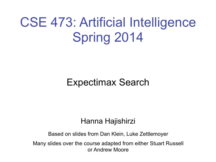
CSE 473: Artificial Intelligence Spring 2014 
 Expectimax Search � � Hanna Hajishirzi Based on slides from Dan Klein, Luke Zettlemoyer Many slides over the course adapted from either Stuart Russell or Andrew Moore 1

Overview: Search

Search Problems Pancake Example: 
 State space graph with costs as weights 4 2 3 2 3 4 3 4 2 3 2 2 3 4 3

General Tree Search Path to reach goal: Flip four, flip three Total cost: 7

Search Strategies § Uninformed Search algorithms: § Depth First Search § Breath First Search § Uniform Cost Search: select smallest g(n) § Heuristic Search: § Best First Search : select smallest h(n) § A* Search: select smallest f(n)=g(n)+h(n) § Graph Search 5

Which Algorithm?

Which Algorithm?

Optimal A* Tree Search § A* tree search is optimal if h is admissible § A heuristic h is admissible (optimistic) if: � where is the true cost to a nearest goal 15

Optimal A* Graph Search § A* graph search is optimal if h is consistent h = 8 B 3 g = 10 G A h = 10 � § Consistency for all edges (A,a,B): § h(A) ≤ c(A,a,B) + h(B) Triangular inequality 9

Which Algorithm?

Overview: Adversarial Search 11

Single Agent Game Tree Value#of#a#state:# Non<Terminal#States:# The#best#achievable# outcome#(u)lity)# from#that#state# 8# 2# 0# …# 2# 6# …# 4# 6# Terminal#States:#

Adversarial Game Tree States#Under#Agent’s#Control:# States#Under#Opponent’s#Control:# <8# <5# <10# +8# Terminal#States:#

Minimax Example 3 12 8 2 4 6 14 5 2

Minimax Properties § Optimal? § Yes, against perfect player. Otherwise? max § Time complexity? § O(b m ) min § Space complexity? § O(bm) 10 10 9 100 § For chess, b ≈ 35, m ≈ 100 § Exact solution is completely infeasible § But, do we need to explore the whole tree?

Today § Adversarial Search § Alpha-beta pruning § Evaluation functions § Expectimax � § Reminder: § Programming 1 due in one week! § Programming 2 will be on adversarial search

Alpha-Beta Pruning Example 7 4 2 1 5 6 0 5 9 2 3 α is MAX’s best alternative here or above β is MIN’s best alternative here or above

Alpha-Beta Pruning Example <=3 >=5 3 7 4 2 1 5 6 0 5 9 2 3 α is MAX’s best alternative here or above β is MIN’s best alternative here or above

Alpha-Beta Pruning Example 3 <=0 0 >=5 3 7 4 2 1 5 6 0 5 2 3 α is MAX’s best alternative here or above β is MIN’s best alternative here or above

Alpha-Beta Pruning Example 3 <=2 <=0 0 2 >=5 3 2 1 5 6 0 5 2 3 α is MAX’s best alternative here or above β is MIN’s best alternative here or above

Alpha-Beta Pruning Example 3 <=2 <=0 0 2 >=5 3 2 1 0 5 2 3 α is MAX’s best alternative here or above β is MIN’s best alternative here or above

Alpha-Beta Pruning Properties § This pruning has no effect on final result at the root � § Values of intermediate nodes might be wrong! § but, they are bounds � § Good child ordering improves effectiveness of pruning � § With “perfect ordering”: § Time complexity drops to O(b m/2 ) § Doubles solvable depth! § Full search of, e.g. chess, is still hopeless …

Resource Limits § Cannot search to leaves max 4 § Depth-limited search -2 4 min min § Instead, search a limited depth of tree -1 -2 4 9 § Replace terminal utilities with an eval function for non-terminal positions § e.g., α - β reaches about depth 8 – decent chess program § Guarantee of optimal play is gone § Evaluation function matters § It works better when we have a greater depth look ahead ? ? ? ?

Depth Matters depth 2

Depth Matters depth 10

Evaluation Functions § Function which scores non-terminals § Ideal function: returns the utility of the position § In practice: typically weighted linear sum of features: § e.g. f 1 ( s ) = (num white queens – num black queens), etc.

Bad Evaluation Function

Why Pacman Starves 8 -2 8 § He knows his score will go up by eating the dot now § He knows his score will go up just as much by eating the dot later on § There are no point-scoring opportunities after eating the dot § Therefore, waiting seems just as good as eating

Evaluation for Pacman What features would be good for Pacman?

Evaluation Function

Evaluation Function

Minimax Example No point in trying

Expectimax 3 ply look ahead, ghosts move randomly Wins some of the games

Worst-case vs. Average max min 10 10 9 100 § Uncertain outcomes are controlled by chance not an adversary § Chance nodes are new types of nodes (instead of Min nodes)

Stochastic Single-Player § What if we don’t know what the result of an action will be? E.g., max § In solitaire, shuffle is unknown § In minesweeper, mine locations average § Can do expectimax search § Chance nodes, like actions except the environment controls the action chosen 10 4 5 7 § Max nodes as before § Chance nodes take average (expectation) of value of children

Expectimax Pseudocode def exp-value(state): initialize v = 0 for each successor of state: 1/2 1/6 p = probability(successor) 1/3 v += p * value(successor) return v 5 8 24 7 -12 v = (1/2) (8) + (1/3) (24) + (1/6) (-12) = 10

Maximum Expected Utility § Why should we average utilities? Why not minimax? § Principle of maximum expected utility: an agent should choose the action which maximizes its expected utility, given its knowledge § General principle for decision making § Often taken as the definition of rationality § We’ll see this idea over and over in this course! § Let’s decompress this definition …

Reminder: Probabilities § A random variable represents an event whose outcome is unknown A probability distribution is an assignment of weights to outcomes § § Example: traffic on freeway? § Random variable: T = whether there’s traffic § Outcomes: T in {none, light, heavy} § Distribution: P(T=none) = 0.25, P(T=light) = 0.55, P(T=heavy) = 0.20 § Some laws of probability (more later): § Probabilities are always non-negative § Probabilities over all possible outcomes sum to one § As we get more evidence, probabilities may change: § P(T=heavy) = 0.20, P(T=heavy | Hour=8am) = 0.60 § We’ll talk about methods for reasoning and updating probabilities later

What are Probabilities? § Objectivist / frequentist answer: § Averages over repeated experiments § E.g. empirically estimating P(rain) from historical observation § E.g. pacman’s estimate of what the ghost will do, given what it has done in the past § Assertion about how future experiments will go (in the limit) § Makes one think of inherently random events, like rolling dice § Subjectivist / Bayesian answer: § Degrees of belief about unobserved variables § E.g. an agent’s belief that it’s raining, given the temperature § E.g. pacman’s belief that the ghost will turn left, given the state § Often learn probabilities from past experiences (more later) § New evidence updates beliefs (more later)

Uncertainty Everywhere § Not just for games of chance! § I’m sick: will I sneeze this minute? § Email contains “FREE!”: is it spam? § Tooth hurts: have cavity? § 60 min enough to get to the airport? § Robot rotated wheel three times, how far did it advance? § Safe to cross street? (Look both ways!) § Sources of uncertainty in random variables: § Inherently random process (dice, etc) § Insufficient or weak evidence § Ignorance of underlying processes § Unmodeled variables § The world’s just noisy – it doesn’t behave according to plan!

Reminder: Expectations § We can define function f(X) of a random variable X § The expected value of a function is its average value, weighted by the probability distribution over inputs § Example: How long to get to the airport? § Length of driving time as a function of traffic: L(none) = 20, L(light) = 30, L(heavy) = 60 § What is my expected driving time? § Notation: E P(T) [ L(T) ] § Remember, P(T) = {none: 0.25, light: 0.5, heavy: 0.25} § E[ L(T) ] = L(none) * P(none) + L(light) * P(light) + L(heavy) * P(heavy) § E[ L(T) ] = (20 * 0.25) + (30 * 0.5) + (60 * 0.25) = 35

Review: Expectations § Real valued functions of random variables: � � § Expectation of a function of a random variable � � � § Example: Expected value of a fair die roll X f P 1 1/6 1 2 1/6 2 3 1/6 3 4 1/6 4 5 1/6 5 6 1/6 6