CSE 373: Minimum Spanning Trees: Prim and Kruskal Michael Lee - PowerPoint PPT Presentation
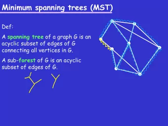
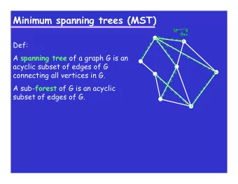
CSE 373: Minimum Spanning Trees: Prim and Kruskal Michael Lee Monday, Feb 26, 2018 1 Minimum spanning trees V ( G is spanning ) ...be undirected. E ). vertex. (Note: this means V ...be connected there is a path from a vertex to any other
Minimum spanning trees: approach 1, adding nodes Intuition: We start with an “empty” MST, and steadily grow it. Core algorithm: 1. Start with an arbitrary node. 2. Run either DFS or BFS, storing edges in our stack or queue. 3. As we visit nodes, add each edge we remove to our MST. 7
Minimum spanning trees: approach 1, adding nodes Intuition: We start with an “empty” MST, and steadily grow it. Core algorithm: 1. Start with an arbitrary node. 2. Run either DFS or BFS, storing edges in our stack or queue. 3. As we visit nodes, add each edge we remove to our MST. 7
Minimum spanning trees: approach 1, adding nodes Intuition: We start with an “empty” MST, and steadily grow it. Core algorithm: 1. Start with an arbitrary node. 2. Run either DFS or BFS, storing edges in our stack or queue. 3. As we visit nodes, add each edge we remove to our MST. 7
Minimum spanning trees: approach 1, adding nodes An example using a modifjed version of DFS: a b d c e f g h i Stack: 8
Minimum spanning trees: approach 1, adding nodes An example using a modifjed version of DFS: a b d c e f g h i 8 Stack: ( a , b ) , ( a , d ) ,
Minimum spanning trees: approach 1, adding nodes An example using a modifjed version of DFS: a b d c e f g h i 8 Stack: ( a , b ) , ( d , e ) , ( d , f ) , ( d , g ) ,
Minimum spanning trees: approach 1, adding nodes An example using a modifjed version of DFS: a b d c e f g h i 8 Stack: ( a , b ) , ( d , e ) , ( d , f ) , ( g , h ) , ( g , i ) ,
Minimum spanning trees: approach 1, adding nodes An example using a modifjed version of DFS: a b d c e f g h i 8 Stack: ( a , b ) , ( d , e ) , ( d , f ) , ( g , h ) ,
Minimum spanning trees: approach 1, adding nodes An example using a modifjed version of DFS: a b d c e f g h i 8 Stack: ( a , b ) , ( d , e ) , ( d , f ) ,
Minimum spanning trees: approach 1, adding nodes An example using a modifjed version of DFS: a b d c e f g h i 8 Stack: ( a , b ) , ( d , e ) ,
Minimum spanning trees: approach 1, adding nodes An example using a modifjed version of DFS: a b d c e f g h i 8 Stack: ( a , b ) , ( e , c ) ,
Minimum spanning trees: approach 1, adding nodes An example using a modifjed version of DFS: a b d c e f g h i 8 Stack: ( a , b ) ,
Minimum spanning trees: approach 1, adding nodes An example using a modifjed version of DFS: a b d c e f g h i Stack: 8
Minimum spanning trees: approach 1, adding nodes What if the edges have difgerent weights? Observation: We solved a similar problem earlier this quarter, when studying shortest path algorithms! 9
Minimum spanning trees: approach 1, adding nodes What if the edges have difgerent weights? Observation: We solved a similar problem earlier this quarter, when studying shortest path algorithms! 9
Interlude: fjnding the shortest path Review: How do we fjnd the shortest path between two vertices? If the graph is weighted: run Dijkstra’s How does Dijkstra’s algorithm work? 1. Give each vertex v a “cost”: the cost of the shortest-known path so far between v and the start. (The cost of a path is the sum of the edge weights in that path) 2. Pick the node with the smallest cost, update adjacent node costs, repeat 10 ◮ If the graph is unweighted: run BFS
Interlude: fjnding the shortest path Review: How do we fjnd the shortest path between two vertices? How does Dijkstra’s algorithm work? 1. Give each vertex v a “cost”: the cost of the shortest-known path so far between v and the start. (The cost of a path is the sum of the edge weights in that path) 2. Pick the node with the smallest cost, update adjacent node costs, repeat 10 ◮ If the graph is unweighted: run BFS ◮ If the graph is weighted: run Dijkstra’s
Interlude: fjnding the shortest path Review: How do we fjnd the shortest path between two vertices? How does Dijkstra’s algorithm work? 1. Give each vertex v a “cost”: the cost of the shortest-known path so far between v and the start. (The cost of a path is the sum of the edge weights in that path) 2. Pick the node with the smallest cost, update adjacent node costs, repeat 10 ◮ If the graph is unweighted: run BFS ◮ If the graph is weighted: run Dijkstra’s
Interlude: fjnding the shortest path Review: How do we fjnd the shortest path between two vertices? How does Dijkstra’s algorithm work? 1. Give each vertex v a “cost”: the cost of the shortest-known path so far between v and the start. (The cost of a path is the sum of the edge weights in that path) 2. Pick the node with the smallest cost, update adjacent node costs, repeat 10 ◮ If the graph is unweighted: run BFS ◮ If the graph is weighted: run Dijkstra’s
Minimum spanning trees: approach 1, adding nodes Intuition: We can use the same idea to fjnd a MST! Core idea: Use the exact same algorithm as Dijkstra’s algorithm, but redefjne the cost: Previously, for Dijkstra’s: The cost of vertex v is the cost of the shortest-known path so far between v and the start Now: The cost of vertex v is the cost of the shortest-known path so far between v and any node we’ve visited so far This algorithm is known as Prim’s algorithm . 11
Minimum spanning trees: approach 1, adding nodes Intuition: We can use the same idea to fjnd a MST! Core idea: Use the exact same algorithm as Dijkstra’s algorithm, but redefjne the cost: The cost of vertex v is the cost of the shortest-known path so far between v and the start Now: The cost of vertex v is the cost of the shortest-known path so far between v and any node we’ve visited so far This algorithm is known as Prim’s algorithm . 11 ◮ Previously, for Dijkstra’s:
Minimum spanning trees: approach 1, adding nodes Intuition: We can use the same idea to fjnd a MST! Core idea: Use the exact same algorithm as Dijkstra’s algorithm, but redefjne the cost: The cost of vertex v is the cost of the shortest-known path so far between v and the start The cost of vertex v is the cost of the shortest-known path so far between v and any node we’ve visited so far This algorithm is known as Prim’s algorithm . 11 ◮ Previously, for Dijkstra’s: ◮ Now:
Minimum spanning trees: approach 1, adding nodes Intuition: We can use the same idea to fjnd a MST! Core idea: Use the exact same algorithm as Dijkstra’s algorithm, but redefjne the cost: The cost of vertex v is the cost of the shortest-known path so far between v and the start The cost of vertex v is the cost of the shortest-known path so far between v and any node we’ve visited so far This algorithm is known as Prim’s algorithm . 11 ◮ Previously, for Dijkstra’s: ◮ Now:
Compare and contrast: Dijkstra vs Prim Pseudocode for Dijkstra’s algorithm: 12 def dijkstra(start): backpointers = new SomeDictionary<Vertex, Vertex>() for (v : vertices): set cost(v) to infinity set cost(start) to 0 while (we still have unvisited nodes): current = get next smallest node for (edge : current.getOutEdges()): newCost = min(cost(current) + edge.cost, cost(edge.dst)) update cost(edge.dst) to newCost backpointers.put(edge.dst, edge.src) return backpointers
Compare and contrast: Dijkstra vs Prim Pseudocode for Prim’s algorithm: 13 def prim(start): backpointers = new SomeDictionary<Vertex, Vertex>() for (v : vertices): set cost(v) to infinity set cost(start) to 0 while (we still have unvisited nodes): current = get next smallest node for (edge : current.getOutEdges()): newCost = min(edge.cost, cost(edge.dst)) update cost(edge.dst) to newCost backpointers.put(edge.dst, edge.src) return backpointers
Prim’s algorithm: an example 11 7 6 1 2 10 14 9 2 4 7 8 a 8 4 i h g f e d c b 14
Prim’s algorithm: an example a 7 6 1 2 10 14 9 2 4 7 11 8 8 4 i 14 d h b g f c e ∞ ∞ ∞ ∞ ∞ ∞ ∞ ∞ ∞ We initially set all costs to ∞ , just like with Dijkstra.
Prim’s algorithm: an example 4 We pick an arbitrary node to start. 7 6 1 2 10 14 9 2 4 7 11 8 8 i a f b c d e g h 14 ∞ ∞ ∞ 0 ∞ ∞ ∞ ∞ ∞
Prim’s algorithm: an example 4 We update the adjacent nodes. 7 6 1 2 10 14 9 2 4 7 11 8 8 i a f b c d e g h 14 4 ∞ ∞ 0 ∞ ∞ ∞ ∞ 8
Prim’s algorithm: an example 4 We select the one with the smallest cost. 7 6 1 2 10 14 9 2 4 7 11 8 8 i a f b c d e g h 14 4 ∞ ∞ 0 ∞ ∞ ∞ ∞ 8
Prim’s algorithm: an example 4 We potentially need to update h and c , but only c changes. 7 6 1 2 10 14 9 2 4 7 11 8 8 i a f b c d e g h 14 4 ∞ 8 0 ∞ ∞ ∞ ∞ 8
Prim’s algorithm: an example 4 We (arbitrarily) pick c . 7 6 1 2 10 14 9 2 4 7 11 8 8 i a f b c d e g h 14 4 8 ∞ ∞ 0 ∞ ∞ ∞ 8
Prim’s algorithm: an example 14 8 11 7 4 2 9 10 4 2 1 6 7 ...and update the adjacent nodes. Note that we don’t add the cumulative cost: the cost represents the shortest path to any green node, not to the start. 8 14 a f b c d i e h g 4 8 7 2 0 ∞ ∞ 8 4
Prim’s algorithm: an example 4 i has the smallest cost. 7 6 1 2 10 14 9 2 4 7 11 8 8 i a f b c d e g h 14 4 7 8 2 0 ∞ ∞ 8 4
Prim’s algorithm: an example 14 8 11 7 4 2 9 10 4 2 1 6 7 We update both unvisited nodes, and modify the edge to h since we now have a better option. 8 14 a f b c d i e h g 4 8 7 2 0 ∞ 7 6 4
Prim’s algorithm: an example 4 f has the smallest cost. 7 6 1 2 10 14 9 2 4 7 11 8 8 i a f b c d e g h 14 4 8 7 2 0 ∞ 7 6 4
Prim’s algorithm: an example 4 Again, we update the adjacent unvisited nodes. 7 6 1 2 10 14 9 2 4 7 11 8 8 i a f b c d e g h 14 4 8 7 2 0 10 7 2 4
Prim’s algorithm: an example 4 g has the smallest cost. 7 6 1 2 10 14 9 2 4 7 11 8 8 i a f b c d e g h 14 4 8 7 2 0 10 7 2 4
Prim’s algorithm: an example 4 We update h again. 7 6 1 2 10 14 9 2 4 7 11 8 8 i a f b c d e g h 14 4 8 7 2 0 10 1 2 4
Prim’s algorithm: an example 4 h has the smallest cost. Note that there nothing to update here. 7 6 1 2 10 14 9 2 4 7 11 8 8 i a f b c d e g h 14 4 8 7 2 0 10 1 2 4
Prim’s algorithm: an example 4 d has the smallest cost. 7 6 1 2 10 14 9 2 4 7 11 8 8 i a f b c d e g h 14 4 7 8 0 2 10 1 2 4
Prim’s algorithm: an example 4 We can update e . 7 6 1 2 10 14 9 2 4 7 11 8 8 i a f b c d e g h 14 4 7 8 0 2 9 1 2 4
Prim’s algorithm: an example 4 e has the smallest cost. 7 6 1 2 10 14 9 2 4 7 11 8 8 i a f b c d e g h 14 4 7 8 0 2 9 1 2 4
Prim’s algorithm: an example 4 There are no more nodes left, so we’re done. 7 6 1 2 10 14 9 2 4 7 11 8 8 i a f b c d e g h 14 4 7 8 0 2 9 2 1 4
Prim’s algorithm: another example Now you try. Start on node a . a b c d e 4 1 2 2 4 3 1 5 15
Prim’s algorithm: another example 1 5 1 3 4 2 2 1 4 e Now you try. Start on node a . 1 d 2 c 2 b 0 a 15
E t u where... Analyzing Prim’s algorithm V log V Fibonacci heaps. if we use E V log V we know how to implement; if we stick to data structures E log V So, Question: What is the worst-case asymptotic runtime of Prim’s time needed to update vertex costs t u time needed to get next smallest node t s V t s Answer: The same as Dijkstra’s: algorithm? 16
Analyzing Prim’s algorithm Question: What is the worst-case asymptotic runtime of Prim’s algorithm? So, V log V E log V if we stick to data structures we know how to implement; V log V E if we use Fibonacci heaps. 16 Answer: The same as Dijkstra’s: O ( | V | t s + | E | t u ) where... ◮ t s = time needed to get next smallest node ◮ t u = time needed to update vertex costs
Analyzing Prim’s algorithm Question: What is the worst-case asymptotic runtime of Prim’s algorithm? Fibonacci heaps. 16 Answer: The same as Dijkstra’s: O ( | V | t s + | E | t u ) where... ◮ t s = time needed to get next smallest node ◮ t u = time needed to update vertex costs So, O ( | V | log ( | V | ) + | E | log ( | V | )) if we stick to data structures we know how to implement; O ( | V | log ( | V | ) + | E | ) if we use
Minimum spanning trees, approach 2 Recap: Prim’s algorithm works similarly to Dijkstra’s – we start with a single node, and “grow” our MST. A second approach: instead of “growing” our MST, we... Initially place each node into its own MST of size 1 – so, we start with V MSTs in total. Steadily combine together difgerent MSTs until we have just one left How? Loop through every single edge, see if we can use it to join two difgerent MSTs together. This algorithm is called Kruskal’s algorithm 17
Minimum spanning trees, approach 2 Recap: Prim’s algorithm works similarly to Dijkstra’s – we start with a single node, and “grow” our MST. A second approach: instead of “growing” our MST, we... Steadily combine together difgerent MSTs until we have just one left How? Loop through every single edge, see if we can use it to join two difgerent MSTs together. This algorithm is called Kruskal’s algorithm 17 ◮ Initially place each node into its own MST of size 1 – so, we start with | V | MSTs in total.
Minimum spanning trees, approach 2 Recap: Prim’s algorithm works similarly to Dijkstra’s – we start with a single node, and “grow” our MST. A second approach: instead of “growing” our MST, we... one left How? Loop through every single edge, see if we can use it to join two difgerent MSTs together. This algorithm is called Kruskal’s algorithm 17 ◮ Initially place each node into its own MST of size 1 – so, we start with | V | MSTs in total. ◮ Steadily combine together difgerent MSTs until we have just
Minimum spanning trees, approach 2 Recap: Prim’s algorithm works similarly to Dijkstra’s – we start with a single node, and “grow” our MST. A second approach: instead of “growing” our MST, we... one left join two difgerent MSTs together. This algorithm is called Kruskal’s algorithm 17 ◮ Initially place each node into its own MST of size 1 – so, we start with | V | MSTs in total. ◮ Steadily combine together difgerent MSTs until we have just ◮ How? Loop through every single edge, see if we can use it to
Kruskal’s algorithm An example, for unweighted graphs. Note: each MST has a difgerent color. a b d c e f g h i 18
Kruskal’s algorithm An example, for unweighted graphs. Note: each MST has a difgerent color. a b d c e f g h i 18
Kruskal’s algorithm An example, for unweighted graphs. Note: each MST has a difgerent color. a b d c e f g h i 18
Kruskal’s algorithm An example, for unweighted graphs. Note: each MST has a difgerent color. a b d c e f g h i 18
Kruskal’s algorithm An example, for unweighted graphs. Note: each MST has a difgerent color. a b d c e f g h i 18
Kruskal’s algorithm An example, for unweighted graphs. Note: each MST has a difgerent color. a b d c e f g h i 18
Kruskal’s algorithm An example, for unweighted graphs. Note: each MST has a difgerent color. a b d c e f g h i 18
Kruskal’s algorithm An example, for unweighted graphs. Note: each MST has a difgerent color. a b d c e f g h i 18
Kruskal’s algorithm An example, for unweighted graphs. Note: each MST has a difgerent color. a b d c e f g h i 18
Kruskal’s algorithm An example, for unweighted graphs. Note: each MST has a difgerent color. a b d c e f g h i 18
Kruskal’s algorithm An example, for unweighted graphs. Note: each MST has a difgerent color. a b d c e f g h i 18
Kruskal’s algorithm An example, for unweighted graphs. Note: each MST has a difgerent color. a b d c e f g h i 18
Kruskal’s algorithm An example, for unweighted graphs. Note: each MST has a difgerent color. a b d c e f g h i 18
Kruskal’s algorithm An example, for unweighted graphs. Note: each MST has a difgerent color. a b d c e f g h i 18
Kruskal’s algorithm An example, for unweighted graphs. Note: each MST has a difgerent color. a b d c e f g h i 18
Kruskal’s algorithm An example, for unweighted graphs. Note: each MST has a difgerent color. a b d c e f g h i 18
Kruskal’s algorithm An example, for unweighted graphs. Note: each MST has a difgerent color. a b d c e f g h i 18
Kruskal’s algorithm An example, for unweighted graphs. Note: each MST has a difgerent color. a b d c e f g h i 18
Kruskal’s algorithm An example, for unweighted graphs. Note: each MST has a difgerent color. a b d c e f g h i 18
Kruskal’s algorithm An example, for unweighted graphs. Note: each MST has a difgerent color. a b d c e f g h i 18
Kruskal’s algorithm An example, for unweighted graphs. Note: each MST has a difgerent color. a b d c e f g h i 18
Kruskal’s algorithm An example, for unweighted graphs. Note: each MST has a difgerent color. a b d c e f g h i 18
Kruskal’s algorithm An example, for unweighted graphs. Note: each MST has a difgerent color. a b d c e f g h i 18
Kruskal’s algorithm An example, for unweighted graphs. Note: each MST has a difgerent color. a b d c e f g h i 18
Kruskal’s algorithm An example, for unweighted graphs. Note: each MST has a difgerent color. a b d c e f g h i 18
Kruskal’s algorithm An example, for unweighted graphs. Note: each MST has a difgerent color. a b d c e f g h i 18
Recommend
More recommend
Explore More Topics
Stay informed with curated content and fresh updates.

