CSE 190 Lecture 16 Data Mining and Predictive Analytics T emporal - PowerPoint PPT Presentation
CSE 190 Lecture 16 Data Mining and Predictive Analytics T emporal data mining This week Temporal models This week well look back on some of the topics already covered in this class, and see how they can be adapted to make use of
CSE 190 – Lecture 16 Data Mining and Predictive Analytics T emporal data mining
This week Temporal models This week we’ll look back on some of the topics already covered in this class, and see how they can be adapted to make use of temporal information 1. Regression – sliding windows and autoregression 2. Classification – dynamic time-warping 3. Dimensionality reduction - ? 4. Recommender systems – some results from Koren Next lecture: 1. Text mining – “Topics over Time” 2. Social networks – densification over time
1. Regression How can we use features such as product properties and user demographics to make predictions about real-valued outcomes (e.g. star ratings)? How can we How can we assess our prevent our decision to models from optimize a overfitting by particular error favouring simpler measure, like the models over more MSE? complex ones?
2. Classification Next we adapted these ideas to binary or multiclass What animal is Will I purchase Will I click on outputs in this image? this product? this ad? Combining features using naïve Bayes models Logistic regression Support vector machines
3. Dimensionality reduction Principal component Community detection analysis
4. Recommender Systems Rating distributions and the missing-not-at-random Latent-factor models assumption
CSE 190 – Lecture 16 Data Mining and Predictive Analytics Regression for sequence data
Week 1 – Regression Given labeled training data of the form Infer the function
Time-series regression Here, we’d like to predict sequences of real-valued events as accurately as possible.
Time-series regression Method 1: maintain a “moving average” using a window of some fixed length
Time-series regression Method 1: maintain a “moving average” using a window of some fixed length • This can be computed efficiently via dynamic programming:
Time-series regression Also useful to plot data: BeerAdvocate, ratings over time BeerAdvocate, ratings over time Sliding window (K=10000) rating rating long-term trends seasonal effects Scatterplot timestamp timestamp Code on: http://jmcauley.ucsd.edu/cse190/code/week10.py
Time-series regression Method 2: weight the points in the moving average by age
Time-series regression Method 3: weight the most recent points exponentially higher
Methods 1, 2, 3 Method 1: Sliding window Method 2: Linear decay Method 3: Exponential decay
Time-series regression Method 4: all of these models are assigning weights to previous values using some predefined scheme, why not just learn the weights?
Time-series regression Method 4: all of these models are assigning weights to previous values using some predefined scheme, why not just learn the weights? • We can now fit this model using least-squares • This procedure is known as autoregression • Using this model, we can capture periodic effects, e.g. that the traffic of a website is most similar to its traffic 7 days ago
CSE 190 – Lecture 16 Data Mining and Predictive Analytics Classification of sequence data
Week 2 How can we predict binary or categorical variables? {0,1}, {True, False} {1, … , N} Another simple algorithm: nearest neighbo(u)rs
Time-series classification As you recall… The longest-common subsequence algorithm is a standard dynamic programming problem - A G C A T 1 st sequence - G A C 2 nd sequence
Time-series classification As you recall… The longest-common subsequence algorithm is a standard dynamic programming problem - A G C A T - A G C A T 1 st sequence - - 0 0 0 0 0 0 G G 0 0 1 1 1 1 A A 0 1 1 1 2 2 C C 0 1 1 2 2 2 = optimal move is to delete from 1 st sequence 2 nd sequence = optimal move is to delete from 2 nd sequence = either deletion is equally optimal = optimal move is a match
Time-series classification The same type of algorithm is used to find correspondences between time-series data (e.g. speech signals), whose length may vary in time/speed DTW_cost = infty for i in range(1,N): for j in range(1,M): d = dist(s[i], t[j]) # Distance between sequences s and t and points i and j skip from seq. 1 DTW[i,j] = d + min(DTW[i-1, j ], skip from seq. 2 DTW[i, j-1], DTW[i-1, j-1] match return DTW[N,M] output is a distance between the two sequences
Time-series classification • This is a simple procedure to infer the similarity between sequences, so we could classify them (for example) using nearest- neighbours (i.e., by comparing a sequence to others with known labels) • We’ll come back to classification soon when we look at time series using graphical models
CSE 190 – Lecture 16 Data Mining and Predictive Analytics T emporal recommender systems
Week 4/5 Recommender Systems go beyond the methods we’ve seen so far by trying to model the relationships between people and the items they’re evaluating my (user’s) HP’s (item) preference is the movie “preferences” “properties” Toward action- “action” heavy? Compatibility preference toward are the special effects good? “special effects”
Week 4/5 Predict a user’s rating of an item according to: By solving the optimization problem: error regularizer (e.g. using stochastic gradient descent)
T emporal latent-factor models To build a reliable system (and to win the Netflix prize!) we need to account for temporal dynamics: Netflix ratings over time Netflix ratings by movie age (Netflix changed their (People tend to give higher ratings to interface) older movies) So how was this actually done? Figure from Koren : “Collaborative Filtering with Temporal Dynamics” (KDD 2009)
T emporal latent-factor models To start with, let’s just assume that it’s only the bias terms that explain these types of temporal variation (which, for the examples on the previous slides, is potentially enough) Idea: temporal dynamics for items can be explained by long- term, gradual changes, whereas for users we’ll need a different model that allows for “ bursty ”, short -lived behavior
T emporal latent-factor models temporal bias model: For item terms, just separate the dataset into (equally sized) bins:* *in Koren’s paper they suggested ~30 bins corresponding to about 10 weeks each for Netflix or bins for periodic effects (e.g. the day of the week): What about user terms? • We need something much finer-grained • But – for most users we have far too little data to fit very short term dynamics
T emporal latent-factor models Start with a simple model of drifting dynamics for users: mean rating hyperparameter date for user u (ended up as x=0.4 for Koren) days away from before (-1) or after mean date (1) the mean date
T emporal latent-factor models Start with a simple model of drifting dynamics for users: mean rating hyperparameter date for user u (ended up as x=0.4 for Koren) days away from before (-1) or after mean date (1) the mean date time-dependent user bias can then be defined as: overall sign and scale for user bias deviation term
T emporal latent-factor models Netflix ratings over time Real data Fitted model
T emporal latent-factor models time-dependent user bias can then be defined as: overall sign and scale for user bias deviation term • Requires only two parameters per user and captures some notion of temporal “drift” (even if the model found through cross-validation is (to me) completely unintuitive) • To develop a slightly more expressive model, we can interpolate smoothly between biases using splines control points
T emporal latent-factor models number of control user bias associated points for this user with this control point (k_u = n_u^0.25 in Koren) time associated with control point (uniformly spaced)
T emporal latent-factor models number of control user bias associated points for this user with this control point (k_u = n_u^0.25 in Koren) time associated with control point (uniformly spaced) • This is now a reasonably flexible model, but still only captures gradual drift , i.e., it can’t handle sudden changes (e.g. a user simply having a bad day)
T emporal latent-factor models • Koren got around this just by adding a “per - day” user bias: bias for a particular day (or session) • Of course, this is only useful for particular days in which users have a lot of (abnormal) activity • The final (time-evolving bias) model then combines all of these factors: global gradual item gradual deviation item bias offset (or splines) bias drift user bias single-day dynamics
T emporal latent-factor models Finally, we can add a time-dependent scaling factor: also defined as Latent factors can also be defined to evolve in the same way: factor-dependent factor-dependent user drift short-term effects
Recommend
More recommend
Explore More Topics
Stay informed with curated content and fresh updates.
