Creating LaTeX and HTML documents from within Stata using texdoc and - PDF document

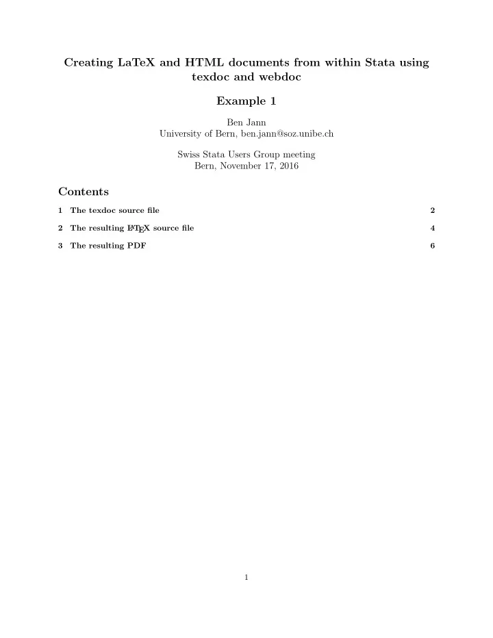
Creating LaTeX and HTML documents from within Stata using texdoc and webdoc Example 1 Ben Jann University of Bern, ben.jann@soz.unibe.ch Swiss Stata Users Group meeting Bern, November 17, 2016 Contents 1 The texdoc source file 2 2 The resulting L A T EX source file 4 3 The resulting PDF 6 1

1 The texdoc source file — the-auto-data.texdoc — texdoc init the-auto-data, replace logdir(log) /// gropts(optargs(width=0.8\textwidth)) set linesize 100 /*** \documentclass[12pt]{article} \usepackage{fullpage} \usepackage{hyperref,graphicx,booktabs,dcolumn} \usepackage{stata} \title{The Auto Data} \author{Ben Jann} \date{\today} \begin{document} \maketitle \begin{abstract} I really like the auto data because it is so awesome. You can do all kinds of stuff with the auto data, like tabulating a variable or computing descriptive statistics. You can even use the auto data to estimate regression models. I am really amazed by the richness of this dataset. There is information on many different makes and models and you can learn, for example, about the gear ratio of a Dodge Diplomat (a stunning 2.47). In this article I will illustrate the auto data and I will show you what you can do with it. I am convinced that you will love this dataset as much as I do after having read this paper. \end{abstract} \tableofcontents \section{Introduction} What we want to do in the introductory section is to open the data and have a look at what is inside of it. Since the auto data is shipped with Stata, we can use the \stcmd{sysuse} command to open it (see \dref{sysuse}). Furthermore, the \stcmd{describe} command will list the variables and display some other information (see \dref{describe}). So let's start: ***/ texdoc stlog sysuse auto texdoc stlog cnp describe texdoc stlog close texdoc local N = r(N) 2

/*** Wow! `N' observations! And what a wealth of variables! Make, price, miles per gallon, and many more. I am very motivated to learn more about this amazing data set. \section{Descriptives} Let's now look at some descriptive statistics. Maybe also let's do a graph. ***/ texdoc stlog summarize pspline price weight texdoc stlog close texdoc local pval = strofreal(r(gof_p),"%9.3f") texdoc graph, label(fig1) caption(What a crazy relation between price and weight) /*** In figure~\ref{fig1} we see that for some unknown reason expensive cars seem to be heavier. Furthermore, the relation appears to be nonlinear, as the pilot goodness-of-fit test rejects the linear fit with a p-value of `pval'. \begin{quote}\small Actually, I really only want to print a graph without printing the code that produced the code. Hm, how can we do that? Maybe the \stcmd{nolog} option will do. \end{quote} ***/ texdoc stlog, nolog pspline price mpg texdoc stlog close texdoc graph, label(fig2) caption(Another crazy relation) /*** In figure~\ref{fig2} we see that price is also related to miles per gallon. How interesting! \section{Regression tables} ***/ texdoc stlog, nolog sysuse auto 3

regress price weight estimates store m1 regress price weight mpg estimates store m2 regress price weight mpg foreign estimates store m3 texdoc local coef = strofreal(_b[weight],"%9.1f") esttab m1 m2 m3 using log/table1.tex, replace se label /// nomtitles booktabs align(D{.}{.}{-1}) /// title(Some regression table\label{table1}) texdoc stlog close /*** Finally we get to regressions! In model~3 of table~\ref{table1} we see that an additional pound of car costs around `coef' dollars once we control for milage and origin. ***/ texdoc write \input{log/table1.tex} /*** \end{document} ***/ — end of file — 2 The resulting L A T EX source file Applying . texdoc do the-auto-data.texdoc generates to the following L A T EX file. — the-auto-data.tex — \documentclass[12pt]{article} \usepackage{fullpage} \usepackage{hyperref,graphicx,booktabs,dcolumn} \usepackage{stata} \title{The Auto Data} \author{Ben Jann} \date{\today} \begin{document} \maketitle \begin{abstract} 4

I really like the auto data because it is so awesome. You can do all kinds of stuff with the auto data, like tabulating a variable or computing descriptive statistics. You can even use the auto data to estimate regression models. I am really amazed by the richness of this dataset. There is information on many different makes and models and you can learn, for example, about the gear ratio of a Dodge Diplomat (a stunning 2.47). In this article I will illustrate the auto data and I will show you what you can do with it. I am convinced that you will love this dataset as much as I do after having read this paper. \end{abstract} \tableofcontents \section{Introduction} What we want to do in the introductory section is to open the data and have a look at what is inside of it. Since the auto data is shipped with Stata, we can use the \stcmd{sysuse} command to open it (see \dref{sysuse}). Furthermore, the \stcmd{describe} command will list the variables and display some other information (see \dref{describe}). So let's start: \begin{stlog}\input{log/1.log.tex}\end{stlog} Wow! 74 observations! And what a wealth of variables! Make, price, miles per gallon, and many more. I am very motivated to learn more about this amazing data set. \section{Descriptives} Let's now look at some descriptive statistics. Maybe also let's do a graph. \begin{stlog}\input{log/2.log.tex}\end{stlog} \begin{figure} \centering \includegraphics[width=0.8\textwidth]{log/2.pdf} \caption{What a crazy relation between price and weight} \label{fig1} \end{figure} In figure~\ref{fig1} we see that for some unknown reason expensive cars seem to be heavier. Furthermore, the relation appears to be nonlinear, as the pilot goodness-of-fit test rejects the linear fit with a p-value of 0.009. \begin{quote}\small Actually, I really only want to print a graph without printing the code that produced the code. Hm, how can we do that? Maybe the \stcmd{nolog} option will do. \end{quote} \begin{figure} 5

\centering \includegraphics[width=0.8\textwidth]{log/3.pdf} \caption{Another crazy relation} \label{fig2} \end{figure} In figure~\ref{fig2} we see that price is also related to miles per gallon. How interesting! \section{Regression tables} Finally we get to regressions! In model~3 of table~\ref{table1} we see that an additional pound of car costs around 3.5 dollars once we control for milage and origin. \input{log/table1.tex} \end{document} — end of file — 3 The resulting PDF The following pages display the resulting PDF after compiling the L A T EX source file. 6

The Auto Data Ben Jann November 17, 2016 Abstract I really like the auto data because it is so awesome. You can do all kinds of stu ff with the auto data, like tabulating a variable or computing descriptive statistics. You can even use the auto data to estimate regression models. I am really amazed by the richness of this dataset. There is information on many di ff erent makes and models and you can learn, for example, about the gear ratio of a Dodge Diplomat (a stunning 2.47). In this article I will illustrate the auto data and I will show you what you can do with it. I am convinced that you will love this dataset as much as I do after having read this paper. Contents 1 Introduction 1 2 Descriptives 2 3 Regression tables 4 1 Introduction What we want to do in the introductory section is to open the data and have a look at what is inside of it. Since the auto data is shipped with Stata, we can use the sysuse command to open it (see [ D ] sysuse ). Furthermore, the describe command will list the variables and display some other information (see [ D ] describe ). So let’s start: . sysuse auto (1978 Automobile Data) 1