CpG Islands - (Durbin Ch.3) In human genomes the C nucleotide of a - PowerPoint PPT Presentation
1 CpG Islands - (Durbin Ch.3) In human genomes the C nucleotide of a dinucleotide CG is typically methylated Methyl-C has a high chance of mutating into a T Thus the dinucleotide CG (CpG) is under-represented Methylation is
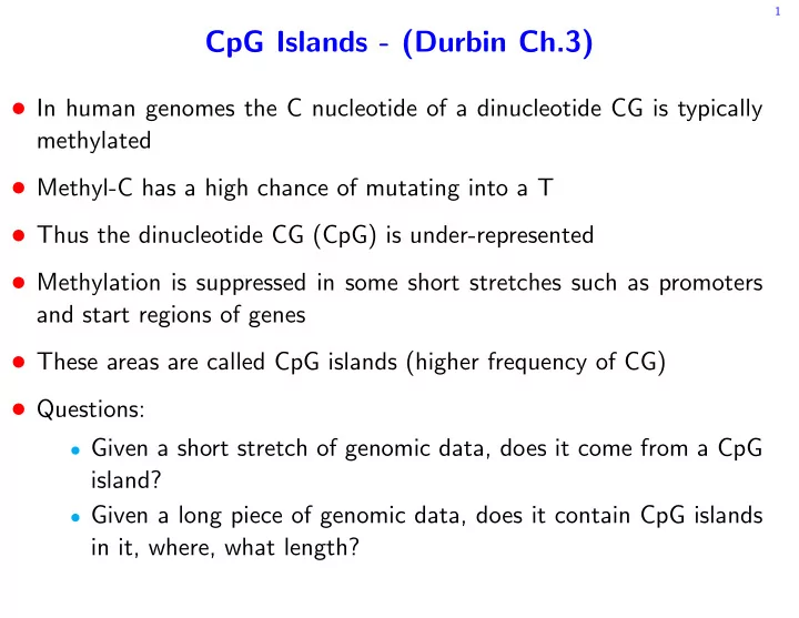
1 CpG Islands - (Durbin Ch.3) • In human genomes the C nucleotide of a dinucleotide CG is typically methylated • Methyl-C has a high chance of mutating into a T • Thus the dinucleotide CG (CpG) is under-represented • Methylation is suppressed in some short stretches such as promoters and start regions of genes • These areas are called CpG islands (higher frequency of CG) • Questions: • Given a short stretch of genomic data, does it come from a CpG island? • Given a long piece of genomic data, does it contain CpG islands in it, where, what length?
2 General decoding problem • Common theme: given a sequence from a certain alphabet suggest what is it? • gene, coding sequence, promoter area, CpG island . . . • How can we determine if a given sequence x is a CpG island? • Construct two data generating models H 0 (“ocean”) and H 1 (“island”) • which one is more likely to have generated the given data (classification problem)
3 LLR statistic and the Neyman-Pearson lemma • Problem: decide whether a given data was generated under H 0 or H 1 • Solution: compute the LLR statistic S ( x ) = log P H 1 ( x ) P H 0 ( x ) • Classify according to a predetermined threshold ( S ( x ) > s α ) • Neyman-Pearson: this test is optimal if H 0 and H 1 are simple hypotheses (as opposed to composite) • H i is a simple hypothesis if P H 0 ( x ) is well defined • For composite hypotheses the likelihood is replaced by a sup • The optimality of the test: • for a given type I error = probability of falsely rejecting H 0 • the type II error = probability of falsely accepting H 0 is minimized
4 Modeling CpG Islands - I • For example, we can set both H 0 and H 1 to be Markov chains with different parametrization (transition probabilities) • Learn the parameters from an annotated sample • if the sample is big enough use ML estimators: c + a + st st := � t ′ c + st ′ • otherwise, smooth using a prior (add dummy counts) • Based on 60,000 nucleotides: + A C G T 0 A C G T A .18 .27 .43 .12 A .30 .20 .29 .21 C .17 .37 .27 .19 C .32 .30 .08 .30 G .16 .34 .38 .12 G .25 .25 .30 .20 T . . . T . . .
5 Modeling CpG Islands - I (cont.) • Using the LLR statistic we have a + S ( x ) = log P H 1 ( x ) � � x i − 1 x i P H 0 ( x ) = log = β x i − 1 x i a − x i − 1 x i i i where x 0 is an artificial start point: a x 0 x 1 = P ( x 1 ) • If S ( x ) > 1 CpG island is more likely, otherwise no CpG island
6 Hidden Markov Models • The occasionally dishonest casino • A casino uses a fair die most of the time � . 5 i = 6 • occasionally switches to a loaded one: p l ( i ) = . 1 i � = 6 • Assume P ( switch to loaded ) = 0 . 05 and P ( switch from loaded ) = 0 . 1 • Let S n denote the die used at the n th roll then SS is a Markov chain • which is hidden from us • we see only the outcomes which could have been “emitted” from either one of the states of the chain • An example of a Hidden Markov Model (HMM)
7 Hidden Markov Models (cont.) • More formally: ( S , X ) is an HMM if S is a Markov chain and P ( X n = x | S , X 1 , . . . , X n − 1 , X n +1 , . . . , X L ) = P ( X n = x | S n ) =: e S n ( x ) • e s ( x ) = P ( X i = x | S i = s ) are called the emission probabilities • Application in communication: • message sent is ( s 1 , . . . , s m ) • received ( x 1 , . . . , x m ) • What is the most likely message sent? • Speech recognition (HMM’s origins) • Claim. The joint probability is given by L � P ( S = s , X = x ) = p ( s , x ) = a s i − 1 s i e s i ( x i ) , i =1
8 HMM for CpG island • States: { + , −} × A , C , T , G • Emissions: e + x ( y ) = e − x ( y ) = 1 x = y • All states are communicating with transition probabilities estimated from annotated sequences • We are interested in decoding a given sequence x : what is the most likely path that generated this sequence • A path automatically yields annotation of CpG islands
9 The Viterbi algorithm • Problem: given the parameters θ = ( a st , e s ) of an HMM and an emitted sequence x , find s ∗ := argmax s P ( S = s | X = x ) • Note that s ∗ = argmax s P ( S = s | X = x ) P ( X = x ) = argmax s p ( s , x ) • Let E ik ( s , x ) := { S 1: i = ( s 1: i − 1 , k ) , X 1: i = x 1: i } and let v k ( i ) := max s P [ E ik ( s , x )] • Claim. v l ( i + 1) = e l ( x i +1 ) max k ( v k ( i ) a kl ) • Note that this is a constructive recursive claim
10 The Viterbi algorithm (cont.) • We add the special initial state 0 • Initialization: v 0 (0) = 1 , v k (0) = 0 for k > 0 • For i = 1 . . . L do, for each state l : • v l ( i ) = e l ( x i ) max k v k ( i − 1) a kl • ptr i ( l ) = argmax k v k ( i − 1) a kl • Termination: • p ( s ∗ , x ) = max k v k ( L ) • Traceback: • s ∗ L = argmax k v k ( L ) • for i = L, . . . , 2 : s ∗ i − 1 = ptr i ( s ∗ i )
11 The Viterbi algorithm (cont.) � . 5 i = 6 300 rolls of our casino a F L = 0 . 05 , a LF = 0 . 1 , e L ( i ) = . . 1 i � = 6
12 The forward algorithm for computing p ( x ) • We want to compute p ( x ) = � s p ( x , s ) • The number of summands grow exponentially with L • Fortunately we have the forward algorithm based on: • Let E i ( x , k ) := { S i = k, X 1: i = x 1: i } • Claim. f l ( i + 1) = e l ( x i +1 ) � k f k ( i ) a kl • As in the Viterbi case, this is a constructive recursion: • Initialization: f 0 (0) := 1 , f k (0) := 0 for k > 0 • For i = 1 , . . . , L : f l ( i ) = e l ( x i ) � k f k ( i − 1) a kl • Termination: p ( x ) = � k f L ( k ) • By itself the forward algorithm is not that important • However it is an important for decoding: computing P ( S i = k | x ) • e.g.: did you loose your house on a loaded die?
13 Posterior distribution of S i • What is p i ( k | x ) := P ( S i = k | X = x ) ? • Since we know p ( x ) , its suffices to find P ( S i = k, X = x ) : P ( S i = k, X = x ) = P ( S i = k, X 1: i = x 1: i , X i +1: L = x i +1: L ) = P ( S i = k, X 1: i = x 1: i ) × P ( X i +1: L = x i +1: L | S i = k, X 1: i = x 1: i ) = f k ( i ) P ( X i +1: L = x i +1: L | S i = k ) � �� � b k ( i )
14 The backward algorithm • The backward algorithm computes b k ( i ) based on • Claim. b k ( i ) = � l a kl b l ( i + 1) e l ( x i +1 ) • The algorithm: • Initialization: b k ( L ) = 1 (more generally b k ( L ) = a k △ , where △ is a terminating state) • For j = L − 1 , . . . , i : b k ( j ) = � l a kl b l ( j + 1) e l ( x j +1 ) • Finally, p i ( k | x ) = f k ( i ) b k ( i ) p ( x ) • To compute p i ( k | x ) for all i, k , run both the backward and forward algorithms once storing f k ( i ) and b k ( i ) for all i, k . • Complexity: let m be the number of states, space O ( mL ) , time O ( m 2 L )
15 Decoding example p i ( F | x ) for same x 1:300 as in the previous graph. Shaded areas correspond to a loaded die. As before, � . 5 i = 6 a F L = 0 . 05 , a LF = 0 . 1 , e L ( i ) = . . 1 i � = 6
16 More on posterior decoding • More generally we might be interested in the expected value of some function of the path, g ( S ) conditioned on the data x . • For example, if for the CpG HMM g ( s ) = 1 + ( s i ) , then � P ( S i = k + | x ) = P (+ | x ) E [ g ( S ) | x ] = k • Comparing that with P ( −| x ) we can find the most probable labeling for x i • We can do that for every i
17 More on posterior decoding/labeling • This maximal posterior labeling procedure applies more generally when labeling defines a partition of the states • Warning: this is not the same as the most probable global labeling of a given sequence! • In our example the latter is given by the Viterbi algorithm • pp. 60-61 in Durbin compare the two approaches: ⊲ Same FN, posterior predicts more short FP
18 Decoding example p i ( F | x ) for x 1:300 . Shaded areas correspond to a loaded die. Note that a F L = 0 . 01 , a LF = 0 . 1 . Viterbi misses the loaded die altogether!
19 Parameter Estimation for HMMs • An HMM model is defined by the parameters: Θ = { a kl , e k ( b ) : ∀ states k, l and symbols b } • We determine Θ using data, or a training set { x 1 , . . . , x n } , where x j are independent samples generated by the model • The likelihood of Θ given the data is � P ( ∩ j { X j = x j }| Θ) := P Θ ( ∩ j { X j = x j } ) = P Θ ( X j = x j ) j • For better numerical stability we work with log-likelihood � log P Θ ( X j = x j ) l ( x 1 , . . . , x n | Θ) = j • The maximum likelihood estimator of Θ is the value of Θ that maximizes the likelihood given the data.
20 Parameter Estimation for HMMs - special case • Suppose our data is labeled in the sense that in addition to each x j we are given the corresponding path s j • In the CpG model this would correspond to having annotated sequences • Can our framework handle the new data? • Yes, the likelihood of Θ is, as before, the probability of the data assuming it was generated by the “model Θ ”: � log P Θ ( X j = x j , S j = s j ) l ( { x j , s j }| Θ) = j • The addition of the path information turns the ML estimation problem into a trivial one • Analogy: it is easier to compute p ( x | s ) than p ( x )
Recommend
More recommend
Explore More Topics
Stay informed with curated content and fresh updates.
