Counterexample-Guided Polynomial Quantitative Loop Invariants by - PowerPoint PPT Presentation
Counterexample-Guided Polynomial Quantitative Loop Invariants by Lagrange Interpolation Yu-Fang Chen 1 Chih-Duo Hong 1 Bow-Yaw Wang 1 Lijun Zhang 2 Institute of Information Science, Academia Sinica, Taiwan Institute of Software, Chinese Academy
Counterexample-Guided Polynomial Quantitative Loop Invariants by Lagrange Interpolation Yu-Fang Chen 1 Chih-Duo Hong 1 Bow-Yaw Wang 1 Lijun Zhang 2 Institute of Information Science, Academia Sinica, Taiwan Institute of Software, Chinese Academy of Sciences, China April 29 th , 2015, Dagstuhl 1 / 39
What this paper is about? Probabilistic program: • used in randomized algorithms, security privacy, randomized protocols. • may change its computation due to probabilistic choices. • quantitative specifications are needed to reason about program correctness. • specified by numerical functions over program variables. • a numerical function may have different values on different executions. • the expected value of a numerical function is then determined. 2 / 39
What this paper is about? Polynomial invariants for probabilistic programs: • annotations with expectations. • correctness of while loops can be proved by inferring special expectations called the quantitative loop invariants . • finding general quantitative loop invariants is hard. • techniques for generating linear quantitative loop invariants are available. • techniques can be extended to synthesize polynomial invariants. • unclear whether the extended approach is still feasible. 3 / 39
What this paper is about? Polynomial invariants for probabilistic programs: • annotations with expectations. • correctness of while loops can be proved by inferring special expectations called the quantitative loop invariants . • finding general quantitative loop invariants is hard. • techniques for generating linear quantitative loop invariants are available. • techniques can be extended to synthesize polynomial invariants. • unclear whether the extended approach is still feasible. polynomial invariants are hard to synthesize in practice!! 4 / 39
What this paper is about? we develop a Lagrange interpolation-based technique to synthesize polynomial loop invariants for simple loops in probabilistic programs 5 / 39
What this talk is about? The results presented here are based on previous works here: • McIver, A., Morgan, C.C.: Abstraction, refinement and proof for probabilistic systems. Springer (2006) • Katoen, J.P., McIver, A.K., Meinicke, L.A., Morgan, C.C.: Linear-invariant generation for probabilistic programs. In: SAS. Springer (2011) 390406 • Gretz, F., Katoen, J.P., McIver, A.: Prinsys on a quest for probabilistic loop invariants. In: QEST. Springer (2013) 193208 • Gretz, F., Katoen, J.P., McIver, A.: Operational versus weakest pre-expectation semantics for the probabilistic guarded command language. Performance Evaluation 73 (2014) 110132 6 / 39
Outline • Preliminaries • Multivariate Lagrange Interpolation • Interpolation of Loop Invariants • Experimental Results • Conclusion 7 / 39
Definitions • Let x m be a sequence of variables x 1 , x 2 , . . . , x m . • We use R [ x n m ] to denote the set of real coefficient polynomials over m variables of degree at most n . • If e 1 , e 2 , . . . , e m are expressions, f ( e 1 , e 2 , . . . , e m ) denotes the polynomial obtained by replacing x i with e i for 1 ≤ i ≤ m in f . • Particularly, f ( v ) is the value of f at v ∈ R m . 8 / 39
Definitions • Let x m be a sequence of variables x 1 , x 2 , . . . , x m . • We use R [ x n m ] to denote the set of real coefficient polynomials over m variables of degree at most n . • If e 1 , e 2 , . . . , e m are expressions, f ( e 1 , e 2 , . . . , e m ) denotes the polynomial obtained by replacing x i with e i for 1 ≤ i ≤ m in f . • Particularly, f ( v ) is the value of f at v ∈ R m . � m + n Observe that R [ x n � m ] can be seen as a vector space over R of dimension d = . n For instance, the set of d monomials { x d 1 1 x d 2 2 · · · x d m m : 0 ≤ d 1 + d 2 + · · · + d m ≤ n } forms a basis of R [ x n m ]. 9 / 39
Probabilistic Programs A probabilistic program in the probabilistic guarded command language is of the following form: P ::= skip | abort | x := E | P ; P | P [ p ] P | if ( G ) then { P } else { P } | while ( G ) { P } where E is an expression and G is a Boolean expression. 10 / 39
Expectations • an expectation is a function mapping program states to a nonnegative real number. • post-expectation : when it is to be evaluated on final program states. • pre-expectation : when it is to be evaluated on initial program states. 11 / 39
Expectations • an expectation is a function mapping program states to a nonnegative real number. • post-expectation : when it is to be evaluated on final program states. • pre-expectation : when it is to be evaluated on initial program states. Definition Let preE and postE be expectations, and prog a probabilistic program. We say a quantitative Hoare triple � preE � prog � postE � holds if the expected value of postE before executing prog is greater than or equal to preE . Note that the expected values of postE and preE are functions over states and hence are compared pointwisely. 12 / 39
Expectations Consider an qualitative Hoare triple { P } prog { Q } with a pre-condition P , a post-condition Q , and a classical program prog : • For any Boolean expression G , define the indicator function [ G ] = 1 if G is true and [ G ] = 0 otherwise. • { P } prog { Q } holds if and only if � [ P ] � prog � [ Q ] � holds. Expectations are therefore the quantitative analogue to predicates for classical programs. 13 / 39
Expectation Transformer for Probabilistic Programs Define the expectation transformer wp ( · , g ) as follows: wp (skip , g ) = g wp (abort , g ) = 0 wp ( x := E , g ) = g [ x / E ] wp ( P ; Q , g ) = wp ( P , wp ( Q , g )) wp (if ( G ) then { P } else { Q } , g ) = [ G ] · wp ( P , g ) + [ ¬ G ] · wp ( Q , g ) wp ( P [ p ] Q , g ) = p · wp ( P , g ) + (1 − p ) · wp ( Q , g ) wp (while ( G ) { P } , g ) = µ X . ([ G ] · wp ( P , X ) + [ ¬ G ] · g ) . 14 / 39
Expectation Transformer for Probabilistic Programs Define the expectation transformer wp ( · , g ) as follows: wp (skip , g ) = g wp (abort , g ) = 0 wp ( x := E , g ) = g [ x / E ] wp ( P ; Q , g ) = wp ( P , wp ( Q , g )) wp (if ( G ) then { P } else { Q } , g ) = [ G ] · wp ( P , g ) + [ ¬ G ] · wp ( Q , g ) wp ( P [ p ] Q , g ) = p · wp ( P , g ) + (1 − p ) · wp ( Q , g ) wp (while ( G ) { P } , g ) = µ X . ([ G ] · wp ( P , X ) + [ ¬ G ] · g ) . • The least fixed point operator µ is defined over the domain of expectations. • It can be shown that � f � P � g � if and only if f ≤ wp ( P , g ). • That is, wp ( P , g ) is the greatest lower bound of pre-expectation of P with respect to g . • We say wp ( P , g ) is the weakest pre-expectation of P with respect to g . 15 / 39
Quantitative Loop Invariants To avoid fixed point computation, we can solve the problem by finding quantitative loop invariants: Theorem Let preE be a pre-expectation, postE a post-expectation, G a Boolean expression, and body a loop-free probabilistic program. To show � preE � while ( G ) { body } � postE � , it suffices to find a loop invariant I which is an expectation such that 1 ( boundary ) preE ≤ I and I · [ ¬ G ] ≤ postE; 2 ( invariant ) I · [ G ] ≤ wp ( body , I ) ; 3 ( soundness ) the loop terminates from any state in G with probability 1 , and 1 the number of iterations is finite; 2 I is bounded above by some fixed constant; or 3 the expected value of I · [ G ] tends to zero as the loop continues to iterate. 16 / 39
Example Example Consider the following probabilistic program (bounded random walk): z := 0; while (0 < x < y ) { x := x + 1 [0 . 5] x := x − 1; z := z + 1; } • It can be shown that any polynomial expectation satisfying the boundary and invariant conditions is also sound, and thus is a loop invariant. • Observe that the soundness of an loop invariant can be verified independent of the pre- and post-expectations. • We only focus on the boundary and invariant conditions. 17 / 39
Multivariate Lagrange Interpolation Lagrange interpolation is a method to construct an explicit expression for any polynomial in R [ x n m ] by sampling. • Fix a degree n of quantitative loop invariants and number of variables m . � m + n • Let d = � . n • Let { b 1 , b 2 , . . . , b d } = { x d 1 1 x d 2 2 · · · x d m m : d 1 + d 2 + · · · + d m ≤ n } be the set of monomials in R [ x n m ]. 18 / 39
Multivariate Lagrange Interpolation Lagrange interpolation is a method to construct an explicit expression for any polynomial in R [ x n m ] by sampling. • Fix a degree n of quantitative loop invariants and number of variables m . � m + n • Let d = � . n • Let { b 1 , b 2 , . . . , b d } = { x d 1 1 x d 2 2 · · · x d m m : d 1 + d 2 + · · · + d m ≤ n } be the set of monomials in R [ x n m ]. Given d sampling points s 1 , s 2 , . . . , s d ∈ R m , we want to compute a Lagrange basis. 19 / 39
Recommend
More recommend
Explore More Topics
Stay informed with curated content and fresh updates.


