CoSc 450: Programming Paradigms 04 A Calculational Deductive System - PowerPoint PPT Presentation
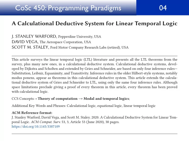
CoSc 450: Programming Paradigms 04 A Calculational Deductive System for Linear Temporal Logic J. STANLEY WARFORD, Pepperdine University, USA DAVID VEGA, The Aerospace Corporation, USA SCOTT M. STALEY, Ford Motor Company Research Labs (retired),
A Calculational Deductive System for Linear Temporal Logic ( σ , j ) | = p U q s 0 s 1 s 2 s 3 s 4 s 5 s 6 s 7 s 8 s 8 ... σ − 1 x 0 1 2 3 4 5 6 7 8 . . . y 9 8 7 6 5 4 3 2 1 0 . . . 0 < x < y F F T T T F F F F F . . . 2 ≤ y < 5 F F F F F T T T F F . . . (0 < x < y ) U (2 ≤ y < 5) F F T T T T T T F F . . . ( ∃ k k ≥ j : ( σ , k ) | = q ∧ ( ∀ i j ≤ i < k : ( σ , i ) | = p ))
A Calculational Deductive System for Linear Temporal Logic ( σ , j ) | = p U q s 0 s 1 s 2 s 3 s 4 s 5 s 6 s 7 s 8 s 8 ... σ − 1 x 0 1 2 3 4 5 6 7 8 . . . y 9 8 7 6 5 4 3 2 1 0 . . . 0 < x < y F F T T T F F F F F . . . 2 ≤ y < 5 F F F F F T T T F F . . . ? (0 < x < y ) U (2 ≤ y < 5) F F T T T T T T F F . . . ( ∃ k k ≥ j : ( σ , k ) | = q ∧ ( ∀ i j ≤ i < k : ( σ , i ) | = p ))
A Calculational Deductive System for Linear Temporal Logic ( σ , j ) | = p U q s 0 s 1 s 2 s 3 s 4 s 5 s 6 s 7 s 8 s 8 ... σ − 1 x 0 1 2 3 4 5 6 7 8 . . . y 9 8 7 6 5 4 3 2 1 0 . . . 0 < x < y F F T T T F F F F F . . . 2 ≤ y < 5 F F F F F T T T F F . . . ? (0 < x < y ) U (2 ≤ y < 5) F F T T T T T T F F . . . What is p U q when k = j, q ≡ true, and p ≡ false? ( ∃ k k ≥ j : ( σ , k ) | = q ∧ ( ∀ i j ≤ i < k : ( σ , i ) | = p ))
A Calculational Deductive System for Linear Temporal Logic ( σ , j ) | = p U q s 0 s 1 s 2 s 3 s 4 s 5 s 6 s 7 s 8 s 8 ... σ − 1 x 0 1 2 3 4 5 6 7 8 . . . y 9 8 7 6 5 4 3 2 1 0 . . . 0 < x < y F F T T T F F F F F . . . 2 ≤ y < 5 F F F F F T T T F F . . . ? (0 < x < y ) U (2 ≤ y < 5) F F T T T T T T F F . . . What is p U q when k = j, q ≡ true, and p ≡ false? ( ∃ k k ≥ j : ( σ , k ) | = q ∧ ( ∀ i j ≤ i < k : ( σ , i ) | = p )) true
A Calculational Deductive System for Linear Temporal Logic ( σ , j ) | = p U q s 0 s 1 s 2 s 3 s 4 s 5 s 6 s 7 s 8 s 8 ... σ − 1 x 0 1 2 3 4 5 6 7 8 . . . y 9 8 7 6 5 4 3 2 1 0 . . . 0 < x < y F F T T T F F F F F . . . 2 ≤ y < 5 F F F F F T T T F F . . . ? (0 < x < y ) U (2 ≤ y < 5) F F T T T T T T F F . . . What is p U q when k = j, q ≡ true, and p ≡ false? ( ∃ k k ≥ j : ( σ , k ) | = q ∧ ( ∀ i j ≤ i < k : ( σ , i ) | = p )) false true
A Calculational Deductive System for Linear Temporal Logic ( σ , j ) | = p U q s 0 s 1 s 2 s 3 s 4 s 5 s 6 s 7 s 8 s 8 ... σ − 1 x 0 1 2 3 4 5 6 7 8 . . . y 9 8 7 6 5 4 3 2 1 0 . . . 0 < x < y F F T T T F F F F F . . . 2 ≤ y < 5 F F F F F T T T F F . . . ? (0 < x < y ) U (2 ≤ y < 5) F F T T T T T T F F . . . What is p U q when k = j, q ≡ true, and p ≡ false? ( ∃ k k ≥ j : ( σ , k ) | = q ∧ ( ∀ i j ≤ i < k : ( σ , i ) | = p )) false false true
A Calculational Deductive System for Linear Temporal Logic ( σ , j ) | = p U q s 0 s 1 s 2 s 3 s 4 s 5 s 6 s 7 s 8 s 8 ... σ − 1 x 0 1 2 3 4 5 6 7 8 . . . y 9 8 7 6 5 4 3 2 1 0 . . . 0 < x < y F F T T T F F F F F . . . 2 ≤ y < 5 F F F F F T T T F F . . . (0 < x < y ) U (2 ≤ y < 5) F F T T T T T T F F . . . The “empty range rule” ( ∃ k k ≥ j : ( σ , k ) | = q ∧ ( ∀ i j ≤ i < k : ( σ , i ) | = p )) false
A Calculational Deductive System for Linear Temporal Logic ( σ , j ) | = p U q s 0 s 1 s 2 s 3 s 4 s 5 s 6 s 7 s 8 s 8 ... σ − 1 x 0 1 2 3 4 5 6 7 8 . . . y 9 8 7 6 5 4 3 2 1 0 . . . 0 < x < y F F T T T F F F F F . . . 2 ≤ y < 5 F F F F F T T T F F . . . (0 < x < y ) U (2 ≤ y < 5) F F T T T T T T F F . . . ( ∃ k k ≥ j : ( σ , k ) | = q ∧ ( ∀ i j ≤ i < k : ( σ , i ) | = p ))
A Calculational Deductive System for Linear Temporal Logic ( σ , j ) | = p U q s 0 s 1 s 2 s 3 s 4 s 5 s 6 s 7 s 8 s 8 ... σ − 1 x 0 1 2 3 4 5 6 7 8 . . . y 9 8 7 6 5 4 3 2 1 0 . . . 0 < x < y F F T T T F F F F F . . . 2 ≤ y < 5 F F F F F T T T F F . . . (0 < x < y ) U (2 ≤ y < 5) F F T T T T T T F F . . . ( ∃ k k ≥ j : ( σ , k ) | = q ∧ ( ∀ i j ≤ i < k : ( σ , i ) | = p ))
A Calculational Deductive System for Linear Temporal Logic ( σ , j ) | = p U q s 0 s 1 s 2 s 3 s 4 s 5 s 6 s 7 s 8 s 8 ... σ − 1 x 0 1 2 3 4 5 6 7 8 . . . y 9 8 7 6 5 4 3 2 1 0 . . . 0 < x < y F F T T T F F F F F . . . 2 ≤ y < 5 F F F F F T T T F F . . . (0 < x < y ) U (2 ≤ y < 5) F F T T T T T T F F . . . ( ∃ k k ≥ j : ( σ , k ) | = q ∧ ( ∀ i j ≤ i < k : ( σ , i ) | = p ))
A Calculational Deductive System for Linear Temporal Logic ( σ , j ) | = p U q s 0 s 1 s 2 s 3 s 4 s 5 s 6 s 7 s 8 s 8 ... σ − 1 x 0 1 2 3 4 5 6 7 8 . . . y 9 8 7 6 5 4 3 2 1 0 . . . 0 < x < y F F T T T F F F F F . . . 2 ≤ y < 5 F F F F F T T T F F . . . (0 < x < y ) U (2 ≤ y < 5) F F T T T T T T F F . . . ( ∃ k k ≥ j : ( σ , k ) | = q ∧ ( ∀ i j ≤ i < k : ( σ , i ) | = p ))
A U B A, B true false � i time ⇥ M. Ben-Ari. Principles of Concurrent and Distributed Programming, Second edition c � M. Ben-Ari 2006 Slide 4.8
A Calculational Deductive System for Linear Temporal Logic The eventually operator � The semantics of the unary prefix operator � is ( � , j ) | = � p ( ⇧ k k ⇤ j : ( � , k ) | = p ) iff s 0 s 1 s 2 s 3 s 4 s 5 s 6 ... σ x 1 2 3 4 5 6 7 . .. 3 ⇥ x < 6 F F T T T F F ... ⇥ (3 ⇥ x < 6) T T T T T F F . .. The bottom row shows the evaluation of the expression where
A Calculational Deductive System for Linear Temporal Logic The eventually operator � The semantics of the unary prefix operator � is ( � , j ) | = � p ( ⇧ k k ⇤ j : ( � , k ) | = p ) iff s 0 s 1 s 2 s 3 s 4 s 5 s 6 ... σ x 1 2 3 4 5 6 7 . .. 3 ⇥ x < 6 F F T T T F F ... ⇥ (3 ⇥ x < 6) T T T T T F F . .. The bottom row shows the evaluation of the expression where
A Calculational Deductive System for Linear Temporal Logic The eventually operator � The semantics of the unary prefix operator � is ( � , j ) | = � p ( ⇧ k k ⇤ j : ( � , k ) | = p ) iff s 0 s 1 s 2 s 3 s 4 s 5 s 6 ... σ x 1 2 3 4 5 6 7 . .. 3 ⇥ x < 6 F F T T T F F ... ⇥ (3 ⇥ x < 6) T T T T T F F . .. The bottom row shows the evaluation of the expression where
A Calculational Deductive System for Linear Temporal Logic The eventually operator � The semantics of the unary prefix operator � is ( � , j ) | = � p ( ⇧ k k ⇤ j : ( � , k ) | = p ) iff s 0 s 1 s 2 s 3 s 4 s 5 s 6 ... σ x 1 2 3 4 5 6 7 . .. 3 ⇥ x < 6 F F T T T F F ... ⇥ (3 ⇥ x < 6) T T T T T F F . .. The bottom row shows the evaluation of the expression where
A Calculational Deductive System for Linear Temporal Logic The eventually operator � The semantics of the unary prefix operator � is ( � , j ) | = � p ( ⇧ k k ⇤ j : ( � , k ) | = p ) iff s 0 s 1 s 2 s 3 s 4 s 5 s 6 ... σ x 1 2 3 4 5 6 7 . .. 3 ⇥ x < 6 F F T T T F F ... ⇥ (3 ⇥ x < 6) T T T T T F F . .. The bottom row shows the evaluation of the expression where
A Calculational Deductive System for Linear Temporal Logic The eventually operator � The semantics of the unary prefix operator � is ( � , j ) | = � p ( ⇧ k k ⇤ j : ( � , k ) | = p ) iff s 0 s 1 s 2 s 3 s 4 s 5 s 6 ... σ x 1 2 3 4 5 6 7 . .. 3 ⇥ x < 6 F F T T T F F ... ⇥ (3 ⇥ x < 6) T T T T T F F . .. The bottom row shows the evaluation of the expression where
A Calculational Deductive System for Linear Temporal Logic The eventually operator � The semantics of the unary prefix operator � is ( � , j ) | = � p ( ⇧ k k ⇤ j : ( � , k ) | = p ) iff s 0 s 1 s 2 s 3 s 4 s 5 s 6 ... σ x 1 2 3 4 5 6 7 . .. 3 ⇥ x < 6 F F T T T F F ... ⇥ (3 ⇥ x < 6) T T T T T F F . .. The bottom row shows the evaluation of the expression where
A Calculational Deductive System for Linear Temporal Logic The eventually operator � The semantics of the unary prefix operator � is ( � , j ) | = � p ( ⇧ k k ⇤ j : ( � , k ) | = p ) iff s 0 s 1 s 2 s 3 s 4 s 5 s 6 ... σ x 1 2 3 4 5 6 7 . .. 3 ⇥ x < 6 F F T T T F F ... ⇥ (3 ⇥ x < 6) T T T T T F F . .. The bottom row shows the evaluation of the expression where
A Calculational Deductive System for Linear Temporal Logic s 0 s 1 s 2 s 3 s 4 s 5 s 6 s 7 s 8 s 9 . . . σ p F F T F F T F F F F ... q F F T T F F T T F F ... ⇥ p T T T T T T F F F F ... ⇥ q T T T T T T T T T T . ..
A Calculational Deductive System for Linear Temporal Logic s 0 s 1 s 2 s 3 s 4 s 5 s 6 s 7 s 8 s 9 . . . σ p F F T F F T F F F F ... q F F T T F F T T F F ... ⇥ p T T T T T T F F F F ... ⇥ q T T T T T T T T T T . ..
A Calculational Deductive System for Linear Temporal Logic s 0 s 1 s 2 s 3 s 4 s 5 s 6 s 7 s 8 s 9 . . . σ p F F T F F T F F F F ... q F F T T F F T T F F ... ⇥ p T T T T T T F F F F ... ⇥ q T T T T T T T T T T . ..
� A A true false � i time ⇥ M. Ben-Ari. Principles of Concurrent and Distributed Programming, Second edition c � M. Ben-Ari 2006 Slide 4.3
� A is a liveness property. Example: p 2 ⇥ � p 4 Algorithm 4.1: Third attempt boolean wantp ⇥ false, wantq ⇥ false p q loop forever loop forever non-critical section non-critical section p1: q1: wantp ⇥ true wantq ⇥ true p2: q2: await wantq = false await wantp = false p3: q3: critical section critical section p4: q4: wantp ⇥ false wantq ⇥ false p5: q5:
A Calculational Deductive System for Linear Temporal Logic The always operator � The semantics of the unary prefix operator � is ( σ , j ) | = � p ( ⌅ k k ⇤ j : ( σ , k ) | = p ) iff s 0 s 1 s 2 s 3 s 4 s 5 s 6 . . . σ x 1 2 3 4 5 6 7 .. . x ⇤ 4 F F F T T T T . . . � ( x ⇤ 4) F F F T T T T . . .
A Calculational Deductive System for Linear Temporal Logic The always operator � The semantics of the unary prefix operator � is ( σ , j ) | = � p ( ⌅ k k ⇤ j : ( σ , k ) | = p ) iff s 0 s 1 s 2 s 3 s 4 s 5 s 6 . . . σ x 1 2 3 4 5 6 7 .. . x ⇤ 4 F F F T T T T . . . � ( x ⇤ 4) F F F T T T T . . .
A Calculational Deductive System for Linear Temporal Logic The always operator � The semantics of the unary prefix operator � is ( σ , j ) | = � p ( ⌅ k k ⇤ j : ( σ , k ) | = p ) iff s 0 s 1 s 2 s 3 s 4 s 5 s 6 . . . σ x 1 2 3 4 5 6 7 .. . x ⇤ 4 F F F T T T T . . . � ( x ⇤ 4) F F F T T T T . . .
A Calculational Deductive System for Linear Temporal Logic The always operator � The semantics of the unary prefix operator � is ( σ , j ) | = � p ( ⌅ k k ⇤ j : ( σ , k ) | = p ) iff s 0 s 1 s 2 s 3 s 4 s 5 s 6 . . . σ x 1 2 3 4 5 6 7 .. . x ⇤ 4 F F F T T T T . . . � ( x ⇤ 4) F F F T T T T . . .
A Calculational Deductive System for Linear Temporal Logic The always operator � The semantics of the unary prefix operator � is ( σ , j ) | = � p ( ⌅ k k ⇤ j : ( σ , k ) | = p ) iff s 0 s 1 s 2 s 3 s 4 s 5 s 6 . . . σ x 1 2 3 4 5 6 7 .. . x ⇤ 4 F F F T T T T . . . � ( x ⇤ 4) F F F T T T T . . .
A Calculational Deductive System for Linear Temporal Logic The always operator � The semantics of the unary prefix operator � is ( σ , j ) | = � p ( ⌅ k k ⇤ j : ( σ , k ) | = p ) iff s 0 s 1 s 2 s 3 s 4 s 5 s 6 . . . σ x 1 2 3 4 5 6 7 .. . x ⇤ 4 F F F T T T T . . . � ( x ⇤ 4) F F F T T T T . . .
A Calculational Deductive System for Linear Temporal Logic The always operator � The semantics of the unary prefix operator � is ( σ , j ) | = � p ( ⌅ k k ⇤ j : ( σ , k ) | = p ) iff s 0 s 1 s 2 s 3 s 4 s 5 s 6 . . . σ x 1 2 3 4 5 6 7 .. . x ⇤ 4 F F F T T T T . . . � ( x ⇤ 4) F F F T T T T . . .
A Calculational Deductive System for Linear Temporal Logic The always operator � The semantics of the unary prefix operator � is ( σ , j ) | = � p ( ⌅ k k ⇤ j : ( σ , k ) | = p ) iff s 0 s 1 s 2 s 3 s 4 s 5 s 6 . . . σ x 1 2 3 4 5 6 7 .. . x ⇤ 4 F F F T T T T . . . � ( x ⇤ 4) F F F T T T T . . .
A Calculational Deductive System for Linear Temporal Logic s 0 s 1 s 2 s 3 s 4 s 5 s 6 s 7 s 8 s 9 ... σ p T T F T T F T T T T . .. q T T F F T T F F T T . .. � p F F F F F F T T T T . .. � q F F F F F F F F F F . ..
A Calculational Deductive System for Linear Temporal Logic s 0 s 1 s 2 s 3 s 4 s 5 s 6 s 7 s 8 s 9 ... σ p T T F T T F T T T T . .. q T T F F T T F F T T . .. � p F F F F F F T T T T . .. � q F F F F F F F F F F . ..
A Calculational Deductive System for Linear Temporal Logic s 0 s 1 s 2 s 3 s 4 s 5 s 6 s 7 s 8 s 9 ... σ p T T F T T F T T T T . .. q T T F F T T F F T T . .. � p F F F F F F T T T T . .. � q F F F F F F F F F F . ..
� A A true false � i time ⇥ M. Ben-Ari. Principles of Concurrent and Distributed Programming, Second edition c � M. Ben-Ari 2006 Slide 4.2
� A is a safety property. Example: � ¬ ( p 4 ⇤ q 4) Algorithm 4.1: Third attempt boolean wantp ⇥ false, wantq ⇥ false p q loop forever loop forever non-critical section non-critical section p1: q1: wantp ⇥ true wantq ⇥ true p2: q2: await wantq = false await wantp = false p3: q3: critical section critical section p4: q4: wantp ⇥ false wantq ⇥ false p5: q5:
To show starvation-free, must prove � ( p 2 ⇥ ⇥ p 4) Algorithm 4.1: Third attempt boolean wantp ⇥ false, wantq ⇥ false p q loop forever loop forever non-critical section non-critical section p1: q1: wantp ⇥ true wantq ⇥ true p2: q2: await wantq = false await wantp = false p3: q3: critical section critical section p4: q4: wantp ⇥ false wantq ⇥ false p5: q5:
Draft (October 31, 2018) 12 2.2.1 Models A model is an infinite anchored sequence [23] of the form where is the initial state and each state is the state at time . For example, suppose is an integer variable whose value varies at each step of the computation. Then, and the expression , known as a state expression, might evolve as follows. ... 8 9 10 11 12 ... F F T T T ... The bottom row shows the evaluation of the state expression for each state in the sequence. Temporal logic extends propositional logic by considering the evolution of expression eval- uations in time. For example, if you assume that in the above sequence keeps increasing by one you can assert informally in English, “For the sequence , eventually will always be true.” The notation means that the expression holds at position in a sequence . In the above example, . The symbol means “satisfies”, so the above expression is read as “State 3 of sequence satisfies .” Or, using “holds”, the same expression is read as, “ holds in state 3 of sequence .” The following sections use to formalize the interpretation of each temporal operator. A Calculational Deductive System for Linear Temporal Logic There is a distinction between the constant true and the truth value of an expression T in a given state. The constant true is an expression that evaluates to T in every state. Similarly, True and False are constants there is a distinction between the constant false and the truth value of an expression F in a given state. The constant false is an expression that evaluates to F in every state. ... s 0 s 1 s 2 s 3 s 4 σ true T T T T T ... false F F F F F ... The propositional logic system of LADM [12] describes a case analysis metatheorem as follows: If and are theorems, then so is . This metatheo- rem does not hold in LTL because the two cases, and , only account for two out of an infinite number of possible sequences of T’s and F’s in .
Draft (October 31, 2018) 12 2.2.1 Models A model is an infinite anchored sequence [23] of the form where is the initial state and each state is the state at time . For example, suppose is an integer variable whose value varies at each step of the computation. Then, and the expression , known as a state expression, might evolve as follows. ... 8 9 10 11 12 ... F F T T T ... The bottom row shows the evaluation of the state expression for each state in the sequence. Temporal logic extends propositional logic by considering the evolution of expression eval- uations in time. For example, if you assume that in the above sequence keeps increasing by one you can assert informally in English, “For the sequence , eventually will always be true.” The notation means that the expression holds at position in a sequence . In the above example, . The symbol means “satisfies”, so the above expression is read as “State 3 of sequence satisfies .” Or, using “holds”, the same expression is read as, “ holds in state 3 of sequence .” The following sections use to formalize the interpretation of each temporal operator. A Calculational Deductive System for Linear Temporal Logic There is a distinction between the constant true and the truth value of an expression T in a given state. The constant true is an expression that evaluates to T in every state. Similarly, True and False are constants there is a distinction between the constant false and the truth value of an expression F in a given state. The constant false is an expression that evaluates to F in every state. ... s 0 s 1 s 2 s 3 s 4 σ true T T T T T ... false F F F F F ... The propositional logic system of LADM [12] describes a case analysis metatheorem as The case analysis metatheorem is NOT valid follows: If and are theorems, then so is . This metatheo- in linear temporal logic! rem does not hold in LTL because the two cases, and , only account for two out of an infinite number of possible sequences of T’s and F’s in .
A Calculational Deductive System for Linear Temporal Logic Next ❡ ❡ ¬ p ≡ ¬ ❡ p (1) Axiom, Self-dual: ❡ over ⇒ : ❡ ( p ⇒ q ) ≡ ❡ p ⇒ ❡ q (2) Axiom, Distributivity of ❡ p ≡ ¬ ❡ ¬ p (3) Linearity: ❡ ❡ ❡ ❡
Draft (November 13, 2014) 18 A Calculational Deductive System for Linear Temporal Logic Here are proofs that ❡ distributes over ∨ , ∧ , and ≡ . Distributivity of ❡ over ∨ : ❡ ( p ∨ q ) ≡ ❡ p ∨ ❡ q (4) Proof : ❡ ( p ∨ q ) = ⟨ (3.59) Implication p ⇒ q ≡ ¬ p ∨ q ⟩ ❡ ( ¬ p ⇒ q ) ⟨ (2) Distributivity of ❡ over ⇒⟩ = ❡ ¬ p ⇒ ❡ q = ⟨ (3.59) Implication p ⇒ q ≡ ¬ p ∨ q with p , q : = ❡ ¬ p , ❡ q ⟩ ¬ ❡ ¬ p ∨ ❡ q = ⟨ (3) Linearity ⟩ ❡ p ∨ ❡ q Distributivity of ❡ over (5) : ❡ ❡ ❡ Proof : (3.12) Double negation, , twice (3.47b) De Morgan, (1) Self-dual with ) (4) Distributivity of over with (1) Self-dual twice (3.47a) De Morgan (3.12) Double negation, (6) Distributivity of over : Proof : Exercise for the student. Hint: Start with mutual implication. Now, holds in the next state, and does not hold in the next state. Theorems (7) and (8) are unique to this system. In equational logic, is theorem (3.4) and is equivalent
Draft (November 13, 2014) 18 A Calculational Deductive System for Linear Temporal Logic Here are proofs that ❡ distributes over ∨ , ∧ , and ≡ . Distributivity of ❡ over ∨ : ❡ ( p ∨ q ) ≡ ❡ p ∨ ❡ q (4) Proof : ❡ ( p ∨ q ) = ⟨ (3.59) Implication p ⇒ q ≡ ¬ p ∨ q ⟩ ❡ ( ¬ p ⇒ q ) ⟨ (2) Distributivity of ❡ over ⇒⟩ = ❡ ¬ p ⇒ ❡ q = ⟨ (3.59) Implication p ⇒ q ≡ ¬ p ∨ q with p , q : = ❡ ¬ p , ❡ q ⟩ ¬ ❡ ¬ p ∨ ❡ q = ⟨ (3) Linearity ⟩ ❡ p ∨ ❡ q Distributivity of ❡ over (5) : ❡ ❡ ❡ Proof : (3.12) Double negation, , twice (3.47b) De Morgan, (1) Self-dual with ) (4) Distributivity of over with (1) Self-dual twice (3.47a) De Morgan (3.12) Double negation, (6) Distributivity of over : Proof : Exercise for the student. Hint: Start with mutual implication. Now, holds in the next state, and does not hold in the next state. Theorems (7) and (8) are unique to this system. In equational logic, is theorem (3.4) and is equivalent
Draft (November 13, 2014) 18 A Calculational Deductive System for Linear Temporal Logic Here are proofs that ❡ distributes over ∨ , ∧ , and ≡ . Distributivity of ❡ over ∨ : ❡ ( p ∨ q ) ≡ ❡ p ∨ ❡ q (4) Proof : ❡ ( p ∨ q ) = ⟨ (3.59) Implication p ⇒ q ≡ ¬ p ∨ q ⟩ ❡ ( ¬ p ⇒ q ) ⟨ (2) Distributivity of ❡ over ⇒⟩ = ❡ ¬ p ⇒ ❡ q = ⟨ (3.59) Implication p ⇒ q ≡ ¬ p ∨ q with p , q : = ❡ ¬ p , ❡ q ⟩ ¬ ❡ ¬ p ∨ ❡ q = ⟨ (3) Linearity ⟩ ❡ p ∨ ❡ q Distributivity of ❡ over (5) : ❡ ❡ ❡ Proof : (3.12) Double negation, , twice (3.47b) De Morgan, (1) Self-dual with ) (4) Distributivity of over with (1) Self-dual twice (3.47a) De Morgan (3.12) Double negation, (6) Distributivity of over : Proof : Exercise for the student. Hint: Start with mutual implication. Now, holds in the next state, and does not hold in the next state. Theorems (7) and (8) are unique to this system. In equational logic, is theorem (3.4) and is equivalent
Draft (November 13, 2014) 18 A Calculational Deductive System for Linear Temporal Logic Here are proofs that ❡ distributes over ∨ , ∧ , and ≡ . Distributivity of ❡ over ∨ : ❡ ( p ∨ q ) ≡ ❡ p ∨ ❡ q (4) Proof : ❡ ( p ∨ q ) = ⟨ (3.59) Implication p ⇒ q ≡ ¬ p ∨ q ⟩ ❡ ( ¬ p ⇒ q ) ⟨ (2) Distributivity of ❡ over ⇒⟩ = ❡ ¬ p ⇒ ❡ q = ⟨ (3.59) Implication p ⇒ q ≡ ¬ p ∨ q with p , q : = ❡ ¬ p , ❡ q ⟩ ¬ ❡ ¬ p ∨ ❡ q = ⟨ (3) Linearity ⟩ ❡ p ∨ ❡ q Distributivity of ❡ over (5) : ❡ ❡ ❡ Proof : (3.12) Double negation, , twice (3.47b) De Morgan, (1) Self-dual with ) (4) Distributivity of over with (1) Self-dual twice (3.47a) De Morgan (3.12) Double negation, (6) Distributivity of over : Proof : Exercise for the student. Hint: Start with mutual implication. Now, holds in the next state, and does not hold in the next state. Theorems (7) and (8) are unique to this system. In equational logic, is theorem (3.4) and is equivalent
Draft (November 13, 2014) 18 A Calculational Deductive System for Linear Temporal Logic Here are proofs that ❡ distributes over ∨ , ∧ , and ≡ . Distributivity of ❡ over ∨ : ❡ ( p ∨ q ) ≡ ❡ p ∨ ❡ q (4) Proof : ❡ ( p ∨ q ) = ⟨ (3.59) Implication p ⇒ q ≡ ¬ p ∨ q ⟩ ❡ ( ¬ p ⇒ q ) ⟨ (2) Distributivity of ❡ over ⇒⟩ = ❡ ¬ p ⇒ ❡ q = ⟨ (3.59) Implication p ⇒ q ≡ ¬ p ∨ q with p , q : = ❡ ¬ p , ❡ q ⟩ ¬ ❡ ¬ p ∨ ❡ q = ⟨ (3) Linearity ⟩ ❡ p ∨ ❡ q Distributivity of ❡ over (5) : ❡ ❡ ❡ Proof : (3.12) Double negation, , twice (3.47b) De Morgan, (1) Self-dual with ) (4) Distributivity of over with (1) Self-dual twice (3.47a) De Morgan (3.12) Double negation, (6) Distributivity of over : Proof : Exercise for the student. Hint: Start with mutual implication. Now, holds in the next state, and does not hold in the next state. Theorems (7) and (8) are unique to this system. In equational logic, is theorem (3.4) and is equivalent
Draft (November 13, 2014) 18 A Calculational Deductive System for Linear Temporal Logic Here are proofs that ❡ distributes over ∨ , ∧ , and ≡ . Distributivity of ❡ over ∨ : ❡ ( p ∨ q ) ≡ ❡ p ∨ ❡ q (4) Proof : ❡ ( p ∨ q ) = ⟨ (3.59) Implication p ⇒ q ≡ ¬ p ∨ q ⟩ ❡ ( ¬ p ⇒ q ) ⟨ (2) Distributivity of ❡ over ⇒⟩ = ❡ ¬ p ⇒ ❡ q = ⟨ (3.59) Implication p ⇒ q ≡ ¬ p ∨ q with p , q : = ❡ ¬ p , ❡ q ⟩ ¬ ❡ ¬ p ∨ ❡ q = ⟨ (3) Linearity ⟩ ❡ p ∨ ❡ q Distributivity of ❡ over (5) : ❡ ❡ ❡ Proof : (3.12) Double negation, , twice (3.47b) De Morgan, (1) Self-dual with ) (4) Distributivity of over with (1) Self-dual twice (3.47a) De Morgan (3.12) Double negation, (6) Distributivity of over : Proof : Exercise for the student. Hint: Start with mutual implication. Now, holds in the next state, and does not hold in the next state. Theorems (7) and (8) are unique to this system. In equational logic, is theorem (3.4) and is equivalent
Draft (November 13, 2014) 18 A Calculational Deductive System for Linear Temporal Logic Here are proofs that ❡ distributes over ∨ , ∧ , and ≡ . Distributivity of ❡ over ∨ : ❡ ( p ∨ q ) ≡ ❡ p ∨ ❡ q (4) Proof : ❡ ( p ∨ q ) = ⟨ (3.59) Implication p ⇒ q ≡ ¬ p ∨ q ⟩ ❡ ( ¬ p ⇒ q ) ⟨ (2) Distributivity of ❡ over ⇒⟩ = ❡ ¬ p ⇒ ❡ q = ⟨ (3.59) Implication p ⇒ q ≡ ¬ p ∨ q with p , q : = ❡ ¬ p , ❡ q ⟩ ¬ ❡ ¬ p ∨ ❡ q = ⟨ (3) Linearity ⟩ ❡ p ∨ ❡ q Distributivity of ❡ over (5) : ❡ ❡ ❡ Proof : (3.12) Double negation, , twice (3.47b) De Morgan, (1) Self-dual with ) (4) Distributivity of over with (1) Self-dual twice (3.47a) De Morgan (3.12) Double negation, (6) Distributivity of over : Proof : Exercise for the student. Hint: Start with mutual implication. Now, holds in the next state, and does not hold in the next state. Theorems (7) and (8) are unique to this system. In equational logic, is theorem (3.4) and is equivalent
Draft (November 13, 2014) 18 A Calculational Deductive System for Linear Temporal Logic Here are proofs that ❡ distributes over ∨ , ∧ , and ≡ . Distributivity of ❡ over ∨ : ❡ ( p ∨ q ) ≡ ❡ p ∨ ❡ q (4) Proof : ❡ ( p ∨ q ) = ⟨ (3.59) Implication p ⇒ q ≡ ¬ p ∨ q ⟩ ❡ ( ¬ p ⇒ q ) ⟨ (2) Distributivity of ❡ over ⇒⟩ = ❡ ¬ p ⇒ ❡ q = ⟨ (3.59) Implication p ⇒ q ≡ ¬ p ∨ q with p , q : = ❡ ¬ p , ❡ q ⟩ ¬ ❡ ¬ p ∨ ❡ q = ⟨ (3) Linearity ⟩ ❡ p ∨ ❡ q Distributivity of ❡ over (5) : ❡ ❡ ❡ Proof : (3.12) Double negation, , twice (3.47b) De Morgan, (1) Self-dual with ) (4) Distributivity of over with (1) Self-dual twice (3.47a) De Morgan (3.12) Double negation, (6) Distributivity of over : Proof : Exercise for the student. Hint: Start with mutual implication. Now, holds in the next state, and does not hold in the next state. Theorems (7) and (8) are unique to this system. In equational logic, is theorem (3.4) and is equivalent
Draft (November 13, 2014) 18 A Calculational Deductive System for Linear Temporal Logic Here are proofs that ❡ distributes over ∨ , ∧ , and ≡ . Distributivity of ❡ over ∨ : ❡ ( p ∨ q ) ≡ ❡ p ∨ ❡ q (4) Proof : ❡ ( p ∨ q ) = ⟨ (3.59) Implication p ⇒ q ≡ ¬ p ∨ q ⟩ ❡ ( ¬ p ⇒ q ) ⟨ (2) Distributivity of ❡ over ⇒⟩ = ❡ ¬ p ⇒ ❡ q = ⟨ (3.59) Implication p ⇒ q ≡ ¬ p ∨ q with p , q : = ❡ ¬ p , ❡ q ⟩ ¬ ❡ ¬ p ∨ ❡ q = ⟨ (3) Linearity ⟩ ❡ p ∨ ❡ q Distributivity of ❡ over (5) : ❡ ❡ ❡ Proof : (3.12) Double negation, , twice (3.47b) De Morgan, (1) Self-dual with ) (4) Distributivity of over with (1) Self-dual twice (3.47a) De Morgan (3.12) Double negation, (6) Distributivity of over : Proof : Exercise for the student. Hint: Start with mutual implication. Now, holds in the next state, and does not hold in the next state. Theorems (7) and (8) are unique to this system. In equational logic, is theorem (3.4) and is equivalent
ACM Computing Surveys submission (August 2019) 20 Linearity follows from self-dual. (3) Linearity: Proof : (3.11) with —(1) Self-dual The proof that distributes over uses the distributivity of over . The proofs that it also distributes over and are similar. (4) Distributivity of over : Proof : (3.59) Implication (2) Distributivity of over (3.59) Implication with A Calculational Deductive System for Linear Temporal Logic (3) Linearity ❡ ∨ ❡ Distributivity of ❡ over ∧ : (5) ❡ ( p ∧ q ) ≡ ❡ p ∧ ❡ q Proof : ❡ ( p ∧ q ) = ⟨ (3.12) Double negation, ¬¬ p ≡ p , twice ⟩ ❡ ( ¬¬ p ∧ ¬¬ q ) = ⟨ (3.47b) De Morgan, ¬ ( p ∨ q ) ≡ ¬ p ∧ ¬ q ⟩ ❡ ¬ ( ¬ p ∨ ¬ q ) = ⟨ (1) Self-dual with p : = ( ¬ p ∨ ¬ q ) ⟩ ¬ ❡ ( ¬ p ∨ ¬ q ) ⟨ (4) Distributivity of ❡ over ∨ with p , q : = ¬ p , ¬ q ⟩ = ¬ ( ❡ ¬ p ∨ ❡ ¬ q ) = ⟨ (3.47b) De Morgan, ¬ ( p ∨ q ) ≡ ¬ p ∧ ¬ q ⟩ ¬ ❡ ¬ p ∧ ¬ ❡ ¬ q = ⟨ (3) Linearity, twice ⟩ ❡ p ∧ ❡ q
ACM Computing Surveys submission (August 2019) 20 Linearity follows from self-dual. (3) Linearity: Proof : (3.11) with —(1) Self-dual The proof that distributes over uses the distributivity of over . The proofs that it also distributes over and are similar. (4) Distributivity of over : Proof : (3.59) Implication (2) Distributivity of over (3.59) Implication with A Calculational Deductive System for Linear Temporal Logic (3) Linearity ❡ ∨ ❡ Distributivity of ❡ over ∧ : (5) ❡ ( p ∧ q ) ≡ ❡ p ∧ ❡ q Proof : ❡ ( p ∧ q ) = ⟨ (3.12) Double negation, ¬¬ p ≡ p , twice ⟩ ❡ ( ¬¬ p ∧ ¬¬ q ) = ⟨ (3.47b) De Morgan, ¬ ( p ∨ q ) ≡ ¬ p ∧ ¬ q ⟩ ❡ ¬ ( ¬ p ∨ ¬ q ) = ⟨ (1) Self-dual with p : = ( ¬ p ∨ ¬ q ) ⟩ ¬ ❡ ( ¬ p ∨ ¬ q ) ⟨ (4) Distributivity of ❡ over ∨ with p , q : = ¬ p , ¬ q ⟩ = ¬ ( ❡ ¬ p ∨ ❡ ¬ q ) = ⟨ (3.47b) De Morgan, ¬ ( p ∨ q ) ≡ ¬ p ∧ ¬ q ⟩ ¬ ❡ ¬ p ∧ ¬ ❡ ¬ q = ⟨ (3) Linearity, twice ⟩ ❡ p ∧ ❡ q
ACM Computing Surveys submission (August 2019) 20 Linearity follows from self-dual. (3) Linearity: Proof : (3.11) with —(1) Self-dual The proof that distributes over uses the distributivity of over . The proofs that it also distributes over and are similar. (4) Distributivity of over : Proof : (3.59) Implication (2) Distributivity of over (3.59) Implication with A Calculational Deductive System for Linear Temporal Logic (3) Linearity ❡ ∨ ❡ Distributivity of ❡ over ∧ : (5) ❡ ( p ∧ q ) ≡ ❡ p ∧ ❡ q Proof : ❡ ( p ∧ q ) = ⟨ (3.12) Double negation, ¬¬ p ≡ p , twice ⟩ ❡ ( ¬¬ p ∧ ¬¬ q ) = ⟨ (3.47b) De Morgan, ¬ ( p ∨ q ) ≡ ¬ p ∧ ¬ q ⟩ ❡ ¬ ( ¬ p ∨ ¬ q ) = ⟨ (1) Self-dual with p : = ( ¬ p ∨ ¬ q ) ⟩ ¬ ❡ ( ¬ p ∨ ¬ q ) ⟨ (4) Distributivity of ❡ over ∨ with p , q : = ¬ p , ¬ q ⟩ = ¬ ( ❡ ¬ p ∨ ❡ ¬ q ) = ⟨ (3.47b) De Morgan, ¬ ( p ∨ q ) ≡ ¬ p ∧ ¬ q ⟩ ¬ ❡ ¬ p ∧ ¬ ❡ ¬ q = ⟨ (3) Linearity, twice ⟩ ❡ p ∧ ❡ q
ACM Computing Surveys submission (August 2019) 20 Linearity follows from self-dual. (3) Linearity: Proof : (3.11) with —(1) Self-dual The proof that distributes over uses the distributivity of over . The proofs that it also distributes over and are similar. (4) Distributivity of over : Proof : (3.59) Implication (2) Distributivity of over (3.59) Implication with A Calculational Deductive System for Linear Temporal Logic (3) Linearity ❡ ∨ ❡ Distributivity of ❡ over ∧ : (5) ❡ ( p ∧ q ) ≡ ❡ p ∧ ❡ q Proof : ❡ ( p ∧ q ) = ⟨ (3.12) Double negation, ¬¬ p ≡ p , twice ⟩ ❡ ( ¬¬ p ∧ ¬¬ q ) = ⟨ (3.47b) De Morgan, ¬ ( p ∨ q ) ≡ ¬ p ∧ ¬ q ⟩ ❡ ¬ ( ¬ p ∨ ¬ q ) = ⟨ (1) Self-dual with p : = ( ¬ p ∨ ¬ q ) ⟩ ¬ ❡ ( ¬ p ∨ ¬ q ) ⟨ (4) Distributivity of ❡ over ∨ with p , q : = ¬ p , ¬ q ⟩ = ¬ ( ❡ ¬ p ∨ ❡ ¬ q ) = ⟨ (3.47b) De Morgan, ¬ ( p ∨ q ) ≡ ¬ p ∧ ¬ q ⟩ ¬ ❡ ¬ p ∧ ¬ ❡ ¬ q = ⟨ (3) Linearity, twice ⟩ ❡ p ∧ ❡ q
ACM Computing Surveys submission (August 2019) 20 Linearity follows from self-dual. (3) Linearity: Proof : (3.11) with —(1) Self-dual The proof that distributes over uses the distributivity of over . The proofs that it also distributes over and are similar. (4) Distributivity of over : Proof : (3.59) Implication (2) Distributivity of over (3.59) Implication with A Calculational Deductive System for Linear Temporal Logic (3) Linearity ❡ ∨ ❡ Distributivity of ❡ over ∧ : (5) ❡ ( p ∧ q ) ≡ ❡ p ∧ ❡ q Proof : ❡ ( p ∧ q ) = ⟨ (3.12) Double negation, ¬¬ p ≡ p , twice ⟩ ❡ ( ¬¬ p ∧ ¬¬ q ) = ⟨ (3.47b) De Morgan, ¬ ( p ∨ q ) ≡ ¬ p ∧ ¬ q ⟩ ❡ ¬ ( ¬ p ∨ ¬ q ) = ⟨ (1) Self-dual with p : = ( ¬ p ∨ ¬ q ) ⟩ ¬ ❡ ( ¬ p ∨ ¬ q ) ⟨ (4) Distributivity of ❡ over ∨ with p , q : = ¬ p , ¬ q ⟩ = ¬ ( ❡ ¬ p ∨ ❡ ¬ q ) = ⟨ (3.47b) De Morgan, ¬ ( p ∨ q ) ≡ ¬ p ∧ ¬ q ⟩ ¬ ❡ ¬ p ∧ ¬ ❡ ¬ q = ⟨ (3) Linearity, twice ⟩ ❡ p ∧ ❡ q
ACM Computing Surveys submission (August 2019) 20 Linearity follows from self-dual. (3) Linearity: Proof : (3.11) with —(1) Self-dual The proof that distributes over uses the distributivity of over . The proofs that it also distributes over and are similar. (4) Distributivity of over : Proof : (3.59) Implication (2) Distributivity of over (3.59) Implication with A Calculational Deductive System for Linear Temporal Logic (3) Linearity ❡ ∨ ❡ Distributivity of ❡ over ∧ : (5) ❡ ( p ∧ q ) ≡ ❡ p ∧ ❡ q Proof : ❡ ( p ∧ q ) = ⟨ (3.12) Double negation, ¬¬ p ≡ p , twice ⟩ ❡ ( ¬¬ p ∧ ¬¬ q ) = ⟨ (3.47b) De Morgan, ¬ ( p ∨ q ) ≡ ¬ p ∧ ¬ q ⟩ ❡ ¬ ( ¬ p ∨ ¬ q ) = ⟨ (1) Self-dual with p : = ( ¬ p ∨ ¬ q ) ⟩ ¬ ❡ ( ¬ p ∨ ¬ q ) ⟨ (4) Distributivity of ❡ over ∨ with p , q : = ¬ p , ¬ q ⟩ = ¬ ( ❡ ¬ p ∨ ❡ ¬ q ) = ⟨ (3.47b) De Morgan, ¬ ( p ∨ q ) ≡ ¬ p ∧ ¬ q ⟩ ¬ ❡ ¬ p ∧ ¬ ❡ ¬ q = ⟨ (3) Linearity, twice ⟩ ❡ p ∧ ❡ q
ACM Computing Surveys submission (August 2019) 20 Linearity follows from self-dual. (3) Linearity: Proof : (3.11) with —(1) Self-dual The proof that distributes over uses the distributivity of over . The proofs that it also distributes over and are similar. (4) Distributivity of over : Proof : (3.59) Implication (2) Distributivity of over (3.59) Implication with A Calculational Deductive System for Linear Temporal Logic (3) Linearity ❡ ∨ ❡ Distributivity of ❡ over ∧ : (5) ❡ ( p ∧ q ) ≡ ❡ p ∧ ❡ q Proof : ❡ ( p ∧ q ) = ⟨ (3.12) Double negation, ¬¬ p ≡ p , twice ⟩ ❡ ( ¬¬ p ∧ ¬¬ q ) = ⟨ (3.47b) De Morgan, ¬ ( p ∨ q ) ≡ ¬ p ∧ ¬ q ⟩ ❡ ¬ ( ¬ p ∨ ¬ q ) = ⟨ (1) Self-dual with p : = ( ¬ p ∨ ¬ q ) ⟩ ¬ ❡ ( ¬ p ∨ ¬ q ) ⟨ (4) Distributivity of ❡ over ∨ with p , q : = ¬ p , ¬ q ⟩ = ¬ ( ❡ ¬ p ∨ ❡ ¬ q ) = ⟨ (3.47b) De Morgan, ¬ ( p ∨ q ) ≡ ¬ p ∧ ¬ q ⟩ ¬ ❡ ¬ p ∧ ¬ ❡ ¬ q = ⟨ (3) Linearity, twice ⟩ ❡ p ∧ ❡ q
ACM Computing Surveys submission (August 2019) 20 Linearity follows from self-dual. (3) Linearity: Proof : (3.11) with —(1) Self-dual The proof that distributes over uses the distributivity of over . The proofs that it also distributes over and are similar. (4) Distributivity of over : Proof : (3.59) Implication (2) Distributivity of over (3.59) Implication with A Calculational Deductive System for Linear Temporal Logic (3) Linearity ❡ ∨ ❡ Distributivity of ❡ over ∧ : (5) ❡ ( p ∧ q ) ≡ ❡ p ∧ ❡ q Proof : ❡ ( p ∧ q ) = ⟨ (3.12) Double negation, ¬¬ p ≡ p , twice ⟩ ❡ ( ¬¬ p ∧ ¬¬ q ) = ⟨ (3.47b) De Morgan, ¬ ( p ∨ q ) ≡ ¬ p ∧ ¬ q ⟩ ❡ ¬ ( ¬ p ∨ ¬ q ) = ⟨ (1) Self-dual with p : = ( ¬ p ∨ ¬ q ) ⟩ ¬ ❡ ( ¬ p ∨ ¬ q ) ⟨ (4) Distributivity of ❡ over ∨ with p , q : = ¬ p , ¬ q ⟩ = ¬ ( ❡ ¬ p ∨ ❡ ¬ q ) = ⟨ (3.47b) De Morgan, ¬ ( p ∨ q ) ≡ ¬ p ∧ ¬ q ⟩ ¬ ❡ ¬ p ∧ ¬ ❡ ¬ q = ⟨ (3) Linearity, twice ⟩ ❡ p ∧ ❡ q
ACM Computing Surveys submission (August 2019) 20 Linearity follows from self-dual. (3) Linearity: Proof : (3.11) with —(1) Self-dual The proof that distributes over uses the distributivity of over . The proofs that it also distributes over and are similar. (4) Distributivity of over : Proof : (3.59) Implication (2) Distributivity of over (3.59) Implication with A Calculational Deductive System for Linear Temporal Logic (3) Linearity ❡ ∨ ❡ Distributivity of ❡ over ∧ : (5) ❡ ( p ∧ q ) ≡ ❡ p ∧ ❡ q Proof : ❡ ( p ∧ q ) = ⟨ (3.12) Double negation, ¬¬ p ≡ p , twice ⟩ ❡ ( ¬¬ p ∧ ¬¬ q ) = ⟨ (3.47b) De Morgan, ¬ ( p ∨ q ) ≡ ¬ p ∧ ¬ q ⟩ ❡ ¬ ( ¬ p ∨ ¬ q ) = ⟨ (1) Self-dual with p : = ( ¬ p ∨ ¬ q ) ⟩ ¬ ❡ ( ¬ p ∨ ¬ q ) ⟨ (4) Distributivity of ❡ over ∨ with p , q : = ¬ p , ¬ q ⟩ = ¬ ( ❡ ¬ p ∨ ❡ ¬ q ) = ⟨ (3.47b) De Morgan, ¬ ( p ∨ q ) ≡ ¬ p ∧ ¬ q ⟩ ¬ ❡ ¬ p ∧ ¬ ❡ ¬ q = ⟨ (3) Linearity, twice ⟩ ❡ p ∧ ❡ q
ACM Computing Surveys submission (August 2019) 20 Linearity follows from self-dual. (3) Linearity: Proof : (3.11) with —(1) Self-dual The proof that distributes over uses the distributivity of over . The proofs that it also distributes over and are similar. (4) Distributivity of over : Proof : (3.59) Implication (2) Distributivity of over (3.59) Implication with A Calculational Deductive System for Linear Temporal Logic (3) Linearity ❡ ∨ ❡ Distributivity of ❡ over ∧ : (5) ❡ ( p ∧ q ) ≡ ❡ p ∧ ❡ q Proof : ❡ ( p ∧ q ) = ⟨ (3.12) Double negation, ¬¬ p ≡ p , twice ⟩ ❡ ( ¬¬ p ∧ ¬¬ q ) = ⟨ (3.47b) De Morgan, ¬ ( p ∨ q ) ≡ ¬ p ∧ ¬ q ⟩ ❡ ¬ ( ¬ p ∨ ¬ q ) = ⟨ (1) Self-dual with p : = ( ¬ p ∨ ¬ q ) ⟩ ¬ ❡ ( ¬ p ∨ ¬ q ) ⟨ (4) Distributivity of ❡ over ∨ with p , q : = ¬ p , ¬ q ⟩ = ¬ ( ❡ ¬ p ∨ ❡ ¬ q ) = ⟨ (3.47b) De Morgan, ¬ ( p ∨ q ) ≡ ¬ p ∧ ¬ q ⟩ ¬ ❡ ¬ p ∧ ¬ ❡ ¬ q = ⟨ (3) Linearity, twice ⟩ ❡ p ∧ ❡ q
ACM Computing Surveys submission (August 2019) 20 Linearity follows from self-dual. (3) Linearity: Proof : (3.11) with —(1) Self-dual The proof that distributes over uses the distributivity of over . The proofs that it also distributes over and are similar. (4) Distributivity of over : Proof : (3.59) Implication (2) Distributivity of over (3.59) Implication with A Calculational Deductive System for Linear Temporal Logic (3) Linearity ❡ ∨ ❡ Distributivity of ❡ over ∧ : (5) ❡ ( p ∧ q ) ≡ ❡ p ∧ ❡ q Proof : ❡ ( p ∧ q ) = ⟨ (3.12) Double negation, ¬¬ p ≡ p , twice ⟩ ❡ ( ¬¬ p ∧ ¬¬ q ) = ⟨ (3.47b) De Morgan, ¬ ( p ∨ q ) ≡ ¬ p ∧ ¬ q ⟩ ❡ ¬ ( ¬ p ∨ ¬ q ) = ⟨ (1) Self-dual with p : = ( ¬ p ∨ ¬ q ) ⟩ ¬ ❡ ( ¬ p ∨ ¬ q ) ⟨ (4) Distributivity of ❡ over ∨ with p , q : = ¬ p , ¬ q ⟩ = ¬ ( ❡ ¬ p ∨ ❡ ¬ q ) = ⟨ (3.47b) De Morgan, ¬ ( p ∨ q ) ≡ ¬ p ∧ ¬ q ⟩ ¬ ❡ ¬ p ∧ ¬ ❡ ¬ q = ⟨ (3) Linearity, twice ⟩ ❡ p ∧ ❡ q
ACM Computing Surveys submission (August 2019) 20 Linearity follows from self-dual. (3) Linearity: Proof : (3.11) with —(1) Self-dual The proof that distributes over uses the distributivity of over . The proofs that it also distributes over and are similar. (4) Distributivity of over : Proof : (3.59) Implication (2) Distributivity of over (3.59) Implication with A Calculational Deductive System for Linear Temporal Logic (3) Linearity ❡ ∨ ❡ Distributivity of ❡ over ∧ : (5) ❡ ( p ∧ q ) ≡ ❡ p ∧ ❡ q Proof : ❡ ( p ∧ q ) = ⟨ (3.12) Double negation, ¬¬ p ≡ p , twice ⟩ ❡ ( ¬¬ p ∧ ¬¬ q ) = ⟨ (3.47b) De Morgan, ¬ ( p ∨ q ) ≡ ¬ p ∧ ¬ q ⟩ ❡ ¬ ( ¬ p ∨ ¬ q ) = ⟨ (1) Self-dual with p : = ( ¬ p ∨ ¬ q ) ⟩ ¬ ❡ ( ¬ p ∨ ¬ q ) ⟨ (4) Distributivity of ❡ over ∨ with p , q : = ¬ p , ¬ q ⟩ = ¬ ( ❡ ¬ p ∨ ❡ ¬ q ) = ⟨ (3.47b) De Morgan, ¬ ( p ∨ q ) ≡ ¬ p ∧ ¬ q ⟩ ¬ ❡ ¬ p ∧ ¬ ❡ ¬ q = ⟨ (3) Linearity, twice ⟩ ❡ p ∧ ❡ q
ACM Computing Surveys submission (August 2019) 20 Linearity follows from self-dual. (3) Linearity: Proof : (3.11) with —(1) Self-dual The proof that distributes over uses the distributivity of over . The proofs that it also distributes over and are similar. (4) Distributivity of over : Proof : (3.59) Implication (2) Distributivity of over (3.59) Implication with A Calculational Deductive System for Linear Temporal Logic (3) Linearity ❡ ∨ ❡ Distributivity of ❡ over ∧ : (5) ❡ ( p ∧ q ) ≡ ❡ p ∧ ❡ q Proof : ❡ ( p ∧ q ) = ⟨ (3.12) Double negation, ¬¬ p ≡ p , twice ⟩ ❡ ( ¬¬ p ∧ ¬¬ q ) = ⟨ (3.47b) De Morgan, ¬ ( p ∨ q ) ≡ ¬ p ∧ ¬ q ⟩ ❡ ¬ ( ¬ p ∨ ¬ q ) = ⟨ (1) Self-dual with p : = ( ¬ p ∨ ¬ q ) ⟩ ¬ ❡ ( ¬ p ∨ ¬ q ) ⟨ (4) Distributivity of ❡ over ∨ with p , q : = ¬ p , ¬ q ⟩ = ¬ ( ❡ ¬ p ∨ ❡ ¬ q ) = ⟨ (3.47b) De Morgan, ¬ ( p ∨ q ) ≡ ¬ p ∧ ¬ q ⟩ ¬ ❡ ¬ p ∧ ¬ ❡ ¬ q = ⟨ (3) Linearity, twice ⟩ ❡ p ∧ ❡ q
A Calculational Deductive System for Linear Temporal Logic Distributivity of � over � : � ( p � q ) � � p � � q (6) Proof: Exercise for the student. Hint: Start with mutual implication.
A Calculational Deductive System for Linear Temporal Logic e true � true (7) Truth of e : Proof: e true = ⇧ (3.28) Excluded middle p ⌅ ¬ p ⌃ e ( p ⌅ ¬ p ) ⇧ (4) Distributivty of e over ⌅⌃ = e p ⌅ e ¬ p = ⇧ (1) Self-dual ⌃ e p ⌅ ¬ e p = ⇧ (3.28) Excluded middle p ⌅ ¬ p with p := e p ⌃ true
A Calculational Deductive System for Linear Temporal Logic e true � true (7) Truth of e : Proof: e true = ⇧ (3.28) Excluded middle p ⌅ ¬ p ⌃ e ( p ⌅ ¬ p ) ⇧ (4) Distributivty of e over ⌅⌃ = e p ⌅ e ¬ p = ⇧ (1) Self-dual ⌃ e p ⌅ ¬ e p = ⇧ (3.28) Excluded middle p ⌅ ¬ p with p := e p ⌃ true
A Calculational Deductive System for Linear Temporal Logic e true � true (7) Truth of e : Proof: e true = ⇧ (3.28) Excluded middle p ⌅ ¬ p ⌃ e ( p ⌅ ¬ p ) ⇧ (4) Distributivty of e over ⌅⌃ = e p ⌅ e ¬ p = ⇧ (1) Self-dual ⌃ e p ⌅ ¬ e p = ⇧ (3.28) Excluded middle p ⌅ ¬ p with p := e p ⌃ true
A Calculational Deductive System for Linear Temporal Logic e true � true (7) Truth of e : Proof: e true = ⇧ (3.28) Excluded middle p ⌅ ¬ p ⌃ e ( p ⌅ ¬ p ) ⇧ (4) Distributivty of e over ⌅⌃ = e p ⌅ e ¬ p = ⇧ (1) Self-dual ⌃ e p ⌅ ¬ e p = ⇧ (3.28) Excluded middle p ⌅ ¬ p with p := e p ⌃ true
A Calculational Deductive System for Linear Temporal Logic e true � true (7) Truth of e : Proof: e true = ⇧ (3.28) Excluded middle p ⌅ ¬ p ⌃ e ( p ⌅ ¬ p ) ⇧ (4) Distributivty of e over ⌅⌃ = e p ⌅ e ¬ p = ⇧ (1) Self-dual ⌃ e p ⌅ ¬ e p = ⇧ (3.28) Excluded middle p ⌅ ¬ p with p := e p ⌃ true
A Calculational Deductive System for Linear Temporal Logic e true � true (7) Truth of e : Proof: e true = ⇧ (3.28) Excluded middle p ⌅ ¬ p ⌃ e ( p ⌅ ¬ p ) ⇧ (4) Distributivty of e over ⌅⌃ = e p ⌅ e ¬ p = ⇧ (1) Self-dual ⌃ e p ⌅ ¬ e p = ⇧ (3.28) Excluded middle p ⌅ ¬ p with p := e p ⌃ true
A Calculational Deductive System for Linear Temporal Logic e true � true (7) Truth of e : Proof: e true = ⇧ (3.28) Excluded middle p ⌅ ¬ p ⌃ e ( p ⌅ ¬ p ) ⇧ (4) Distributivty of e over ⌅⌃ = e p ⌅ e ¬ p = ⇧ (1) Self-dual ⌃ e p ⌅ ¬ e p = ⇧ (3.28) Excluded middle p ⌅ ¬ p with p := e p ⌃ true
A Calculational Deductive System for Linear Temporal Logic e true � true (7) Truth of e : Proof: e true = ⇧ (3.28) Excluded middle p ⌅ ¬ p ⌃ e ( p ⌅ ¬ p ) ⇧ (4) Distributivty of e over ⌅⌃ = e p ⌅ e ¬ p = ⇧ (1) Self-dual ⌃ e p ⌅ ¬ e p = ⇧ (3.28) Excluded middle p ⌅ ¬ p with p := e p ⌃ true
A Calculational Deductive System for Linear Temporal Logic e true � true (7) Truth of e : Proof: e true = ⇧ (3.28) Excluded middle p ⌅ ¬ p ⌃ e ( p ⌅ ¬ p ) ⇧ (4) Distributivty of e over ⌅⌃ = e p ⌅ e ¬ p = ⇧ (1) Self-dual ⌃ e p ⌅ ¬ e p = ⇧ (3.28) Excluded middle p ⌅ ¬ p with p := e p ⌃ true
A Calculational Deductive System for Linear Temporal Logic e false � false (8) Falsehood of e : Proof: Exercise for the student.
A Calculational Deductive System for Linear Temporal Logic Until U ❡ over U : ❡ ( p U q ) ≡ (9) Axiom, Distributivity of ❡ p U ❡ q p U q ≡ q ∨ ( p ∧ ❡ ( p U q )) (10) Axiom, Expansion of U : p U false ≡ false (11) Axiom, Right zero of U : p U ( q ∨ r ) ≡ p U q ∨ p U r (12) Axiom, Left distributivity of U over ∨ : p U r ∨ q U r ⇒ ( p ∨ q ) U r (13) Axiom, Right distributivity of U over ∨ : p U ( q ∧ r ) ⇒ p U q ∧ p U r (14) Axiom, Left distributivity of U over ∧ : ( p ∧ q ) U r ≡ p U r ∧ q U r (15) Axiom, Right distributivity of U over ∧ : (16) Axiom, U implication ordering: p U q ∧ ¬ q U r ⇒ p U r p U ( q U r ) ⇒ ( p ∨ q ) U r (17) Axiom, Right U ∨ ordering: p U ( q ∧ r ) ⇒ ( p U q ) U r (18) Axiom, Right ∧ U ordering:
A Calculational Deductive System for Linear Temporal Logic ∧ ∧ ⇒ ( p ⇒ q ) U r ⇒ ( p U r ⇒ q U r ) (19) Right distributivity of U over ⇒ : (20) Right zero of U : p U true ≡ true false U q ≡ q (21) Left identity of U : (22) Idempotency of U : p U p ≡ p (23) U excluded middle: p U q ∨ p U ¬ q (24) ¬ p U ( q U r ) ∧ p U r ⇒ q U r
Draft (November 14, 2017) 22 with as the left argument is the basis of the definition of the eventually operator in Section 3.3. (20) Right zero of : A Calculational Deductive System for Linear Temporal Logic (21) Left identity of : Theorem (22) shows that the until operator is idempotent. Theorem (23) is the until version of excluded middle. Theorem (28) is interesting because it relates the temporal expression on the left hand side to the propositional expression on the right hand side. (22) Idempotency of U : p U p ≡ p Proof : p U p = ⟨ (10) Expansion of U ⟩ p ∨ ( p ∧ ❡ ( p U p )) = ⟨ (3.43b) Absorption, p ∨ ( p ∧ q ) ≡ p with q : = ❡ ( p U p ) ⟩ p (23) excluded middle: Proof : (Ravi Mohan) (12) Left distributivity of over (3.28) Excluded middle, (20) Right zero of (24) Proof : The proof is by (4.7.1) Truth implication. (17) Right ordering with (3.59) Implication, (19) Right distributivity of over and (3.82a) Transitivity (3.65) Shunting,
Draft (November 14, 2017) 22 with as the left argument is the basis of the definition of the eventually operator in Section 3.3. (20) Right zero of : A Calculational Deductive System for Linear Temporal Logic (21) Left identity of : Theorem (22) shows that the until operator is idempotent. Theorem (23) is the until version of excluded middle. Theorem (28) is interesting because it relates the temporal expression on the left hand side to the propositional expression on the right hand side. (22) Idempotency of U : p U p ≡ p Proof : p U p = ⟨ (10) Expansion of U ⟩ p ∨ ( p ∧ ❡ ( p U p )) = ⟨ (3.43b) Absorption, p ∨ ( p ∧ q ) ≡ p with q : = ❡ ( p U p ) ⟩ p (23) excluded middle: Proof : (Ravi Mohan) (12) Left distributivity of over (3.28) Excluded middle, (20) Right zero of (24) Proof : The proof is by (4.7.1) Truth implication. (17) Right ordering with (3.59) Implication, (19) Right distributivity of over and (3.82a) Transitivity (3.65) Shunting,
Draft (November 14, 2017) 22 with as the left argument is the basis of the definition of the eventually operator in Section 3.3. (20) Right zero of : A Calculational Deductive System for Linear Temporal Logic (21) Left identity of : Theorem (22) shows that the until operator is idempotent. Theorem (23) is the until version of excluded middle. Theorem (28) is interesting because it relates the temporal expression on the left hand side to the propositional expression on the right hand side. (22) Idempotency of U : p U p ≡ p Proof : p U p = ⟨ (10) Expansion of U ⟩ p ∨ ( p ∧ ❡ ( p U p )) = ⟨ (3.43b) Absorption, p ∨ ( p ∧ q ) ≡ p with q : = ❡ ( p U p ) ⟩ p (23) excluded middle: Proof : (Ravi Mohan) (12) Left distributivity of over (3.28) Excluded middle, (20) Right zero of (24) Proof : The proof is by (4.7.1) Truth implication. (17) Right ordering with (3.59) Implication, (19) Right distributivity of over and (3.82a) Transitivity (3.65) Shunting,
Recommend
More recommend
Explore More Topics
Stay informed with curated content and fresh updates.
