Intro to Probabilistic Relational Models James Lenfestey, with Tom - PowerPoint PPT Presentation

Intro to Probabilistic Relational Models James Lenfestey, with Tom Temple and Ethan Howe Intro to Probabilistic Relational Models – p.1/24

Outline � Motivate problem � Define PRMs � Extensions and future work Intro to Probabilistic Relational Models – p.2/24

Our Goal � Observation: the world consists of many distinct entities with similar behaviors � Exploit this redundancy to make our models simpler � This was the idea of FOL: use quantification to eliminate redundant sentences over ground literals Intro to Probabilistic Relational Models – p.3/24

Example: A simple domain � a set of students, S = { s 1 , s 2 , s 3 } � a set of professors, P = { p 1 , p 2 , p 3 } � Well-Funded , Famous : P → { true , f alse } � Student-Of : S × P → { true , f alse } � Successful : S → { true , f alse } Intro to Probabilistic Relational Models – p.4/24

Example: A simple domain We can express a certain self-evident fact in one sentence of FOL: ∀ s ∈ S ∀ p ∈ P Famous ( p ) and Student-Of ( s , p ) ⇒ Successful ( s ) Intro to Probabilistic Relational Models – p.5/24

Example: A simple domain The same sentence converted to propositional logic: ( ¬ ( p 1 _ f amous and student _ o f _ s 1 _ p 1 ) or s 1 _ success f ul ) and ( ¬ ( p 1 _ f amous and student _ o f _ s 2 _ p 1 ) or s 2 _ success f ul ) and ( ¬ ( p 1 _ f amous and student _ o f _ s 3 _ p 1 ) or s 3 _ success f ul ) and ( ¬ ( p 2 _ f amous and student _ o f _ s 1 _ p 1 ) or s 1 _ success f ul ) and ( ¬ ( p 2 _ f amous and student _ o f _ s 2 _ p 1 ) or s 2 _ success f ul ) and ( ¬ ( p 2 _ f amous and student _ o f _ s 3 _ p 1 ) or s 3 _ success f ul ) and ( ¬ ( p 3 _ f amous and student _ o f _ s 1 _ p 1 ) or s 1 _ success f ul ) and ( ¬ ( p 3 _ f amous and student _ o f _ s 2 _ p 1 ) or s 2 _ success f ul ) and ( ¬ ( p 3 _ f amous and student _ o f _ s 3 _ p 1 ) or s 3 _ success f ul ) Intro to Probabilistic Relational Models – p.6/24

Our Goal � Unfortunately, the real world is not so clear-cut � Need a probabilistic version of FOL � Proposal: PRMs Propositional Bayes Logic Nets First-order PRMs Logic Intro to Probabilistic Relational Models – p.7/24

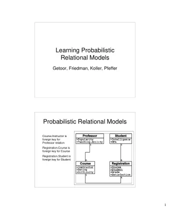
Defining the Schema � The world consists of base entities, partitioned into classes X 1 , X 2 , ..., X n � Elements of these classes share connections via a collection of relations R 1 , R 2 , ..., R m � Each entity type is characterized by a set of attributes, A ( X i ) . Each attribute A j ∈ A ( X i ) assumes values from a fixed domain, V ( A j ) � Defines the schema of a relational model Intro to Probabilistic Relational Models – p.8/24

Continuing the example... We can modify the domain previously given to this new framework: � 2 classes: S , P � 1 relation: Student-Of ⊂ S × P � A ( S ) = { Success } � A ( P ) = { Well-Funded , Famous } Intro to Probabilistic Relational Models – p.9/24

Instantiations An instantiation I of the relational schema defines � a concrete set of base entities O I ( X i ) for each class X i � values for the attributes of each base entity for each class � R i ( X 1 , ..., X k ) ⊂ O I ( X 1 ) × ... × O I ( X k ) for each R i . Intro to Probabilistic Relational Models – p.10/24

Slot chains We can project any relation R ( X 1 , ..., X k ) onto its i th and j th components to obtain a binary relation ρ ( X i , X j ) . Consider this a function mapping instances of X i to sets of instances of X j . That is, for x ∈ O I ( X i ) , let x . ρ = { y ∈ O I ( X j ) | ( x , y ) ∈ ρ ( X i , X j ) } . We call ρ a slot of X i . Composition of slots (via transitive closure) gives a slot chain . Intro to Probabilistic Relational Models – p.11/24

Probabilities, finally � The idea of a PRM is to express a joint probability distribution over all possible instantiations of a particular relational schema � Since there are infinitely many possible instantiations to a given schema, specifying the full joint distribution would be very painful � Instead, compute marginal probabilities over remaining variables given a partial instantiation Intro to Probabilistic Relational Models – p.12/24

Partial Instantiations A partial instantiation I ′ specifies � the sets O I ′ ( X i ) � the relations R j � values of some attributes for some of the base entities The PRM inference problem is to calculate the distribution over values for the unassigned attributes. Intro to Probabilistic Relational Models – p.13/24

Locality of Influence � BNs and PRMs are alike in that they both assume that real-world data exhibits locality of influence , the idea that most variables are influenced by only a few others. � Both models exploit this property through conditional independence . � PRMs go beyond BNs by assuming that there are few distinct patterns of influence in total Intro to Probabilistic Relational Models – p.14/24

Conditional independence � For a class X , values of the attribute X . A are influenced by attributes in the set Pa ( X . A ) (its parents). � Pa ( X . A ) contains attributes of the form X . B ( B an attribute) or X . τ . B ( τ a slot chain). � As in a BN, the value of X . A is conditionally independent of the values of all other attributes, given its parents. Intro to Probabilistic Relational Models – p.15/24

An example Student Student-Of Professor Famous Successful Well-Funded Captures the FOL sentence from before in a proba- bilistic framework. Intro to Probabilistic Relational Models – p.16/24

Compiling into a BN A PRM can be compiled into a BN, just as a statement in FOL can be compiled to a statement in PL. p2_famous p2_well-funded p1_famous p3_famous p1_well-funded p3_well-funded s2_success s1_success s3_success Intro to Probabilistic Relational Models – p.17/24

PRM p2_famous p2_well-funded p1_famous p3_famous p1_well-funded p3_well-funded s2_success s1_success s3_success We can us this network to support inference over queries regarding base entities. Intro to Probabilistic Relational Models – p.18/24

Aggregates � Pa ( X . A ) may contain X . τ . B for slot chain τ , which is generally a multiset. � Pa ( X . A ) dependent on the value of the set, not just the values in the multiset � Representational challenge, again | X . τ . B | has no bound a priori Intro to Probabilistic Relational Models – p.19/24

Aggregates � γ summarizes the contents of X . τ . B � Let γ ( X . τ . B ) be a parent of attributes of X � Many useful aggregates: mean, cardinality, median, etc. � Require computation of γ to be deterministic (we can omit it from the diagram) Intro to Probabilistic Relational Models – p.20/24

Example: Aggregates � Let γ ( A ) = | A | � Let Advisor-Of = Student-Of − 1 � e.g. p 1 . Advisor-Of = { s 1 } , p 2 . Advisor-Of = {} , p 3 . Advisor-Of = { s 2 , s 3 } � To represent the idea that a professor’s funding is influenced by the number of advisees: Pa ( P . Well-Funded ) = {P . Famous , γ ( P . Advisor-Of ) } Intro to Probabilistic Relational Models – p.21/24

Extensions � Reference uncertainty. Not all relations known a priori; may depend probabilistically on values of attributes. E.g., students prefer advisors with more funding. � Identity uncertainty. Distinct entities might not refer to distinct real-world objects. � Dynamic PRMs. Objects and relations change over time; can be unfolded into a DBN at the expense of a very large state space. Intro to Probabilistic Relational Models – p.22/24

Acknowledgements � “Approximate inference for first-order probabilistic languages”, Pasula and Russell. Running example. � “Learning Probabilistic Relational Models”, Friedman et al. Borrowed notation. Intro to Probabilistic Relational Models – p.23/24

Resources � “Approximate inference for first-order probabilistic languages” gives a promising MCMC approach for addressing relational and identity uncertainty. � “Inference in Dynamic Probabilistic Relational Models”, Sanhai et al. Particle-filter based DPRM inference that uses abstraction smoothing to generalize over related objects. Intro to Probabilistic Relational Models – p.24/24