Conversion of MAGIC data to DL3 format L. Jouvin, J. Delgado, C. - PowerPoint PPT Presentation
Conversion of MAGIC data to DL3 format L. Jouvin, J. Delgado, C. Nigro, J. Rico 1 MAGIC At the Roque de los Muchachos Observatory in La Palma Operating since 2004 Since 2009: 2 Imaging Atmospheric Cherenkov telescopes 17 m
Conversion of MAGIC data to DL3 format L. Jouvin, J. Delgado, C. Nigro, J. Rico 1
MAGIC At the Roque de los Muchachos Observatory in La Palma • Operating since 2004 • Since 2009: 2 Imaging Atmospheric Cherenkov telescopes • 17 m diameters • Summers 2011-2012: telescopes underwent a series of upgrades • Sensitive between 50 GeV and 30 TeV • 2
DL3 format DL3 is event lists + IRFs for each observation after applying analysis cuts. Events list : γ-like events ● IRFs : ● Effective area ● Energy resolution ● PSF ● Background ● Two types of IRF: ● – Pointlike – Full 3 θ 0 θ 2
First joint analysis of the Crab Nebula DL3 MAGIC converter ● Perform a multi-instrument spectral analysis of the Crab Nebula with Gammapy ● C. Nigro et al. 4
3D likelihood analysis ● Source morphology: more and more precise and complex ● This complexity will increase with CTA observation ● cube analysis: fit simultaneously the morphology and the spectrum on a cube dataset → required to separate the different components of a same region of the sky For morphological 2D analysis and 3D analysis, we need: → IRF full enclosure (without theta2 cut) → Offset dependant in the FOV → PSF → Background model 5
MAGIC analysis software (MARS) 6
DL3 Event List Melibea level in MARS contain: ● ● Incident Direction ● Energy of the primary gamma-ray ● Hadronness (gamma/hadrons separation) ● Good time interval Created for each run (~20min) of observations, or for MC events. ● Fix a hadronness → event list for this cut ● DL3 level for event lists is the output of the Melibea program ● 7
DL3 IRF ● flute and the DL3 exporter ● flute: Start from data and MC from the melibea level. – Weight IRF by zenith and azimuth distribution of the events → Produce IRF – for each observation condition. Used to compute: – ➢ Effective area in true energy ➢ The effective on time in each bin of azimuth and zenith ➢ List of MC events containing: true and reconstructed energy ● Energy dispersion in DL3 exporter: list of MC events weighting by the effective on time distribution for each run ● Use single offset MC simulation at 0.4° ● Pointlike 8
Main current work in the DL3 group ● General pipeline ● Offset dependent IRF in the FOV ● PSF for each observation ● Full IRF 9
General pipeline for all MC period Summer 2011-2012: telescopes underwent a series of upgrades • 8 MC periods → we want to produce general RFs that covers each • specific MC period deliver complete DL3 release for each MC period • started with one MC period : 2013-07-27 - 2014-06-18 • Most of the observations: pointlike source at 0.4° • 10
Start with one MC period under development with Jordi Delgado • 4 known pointlike sources • Joint Crab paper: 2 runs of 04/10/2013 Specific RF General pipeline phi 1TeV = (4.14 +/- 0.30) 10 -11 cm -2 TeV -1 s -1 phi 1TeV = (4.22 +/- 0.30) 10 -11 cm -2 TeV -1 s -1 Alpha= 2.52 +/- 0.08 α= 2.55 +/- 0.09 β= 0.17 +/- 0.05 Beta= 0.16 +/- 0.04 11
Offset dependent IRF 12
From diffuse MC ● Use diffuse MC ● creating rings at different offset Diffuse Ring MC Select a 0.5° specific ring 0.3° 13 → IRF at 0.4° Different Ring → IRF offset dependant in the FOV
Crab offset dependant observation MC period: 2013-07-27 – 2014-06-18 Offset: Diffuse ring: ● 0.2 ° ● 0 – 0.3 ° ● 0.35 ° ● 0.3 – 0.5 ° ● 0.4 ° ● 0.3 – 0.5 ° ● 0.7 ° ● 0.5 – 0.8 ° ● 1.0 ° ● 0.8 – 1.1 ° ● 1.4 ° ● 1.3 – 1.4 ° 14
Crab Nebula spectrum at different offset → Large offset: camera inhomogeneties, not possible to use reflected region → MAGIC software: correction by the acceptance possible for the background extraction. → Problem with Gammapy that uses only reflected region 15
Flute and DL3 exporter produce IRFs offset dependant Diffuse ring: Offset Median: 0.0 – 0.3 ° 0.22 ° ● ● 0.3 – 0.5° 0.41 ° ● ● Associated FOV offset in the DL3: 0.5 – 0.7 ° 0.6 ° Median of the offset distribution in each ring ● ● 0.7 – 0.9 ° 0.8 ° ● ● 0.9 – 1.1 ° 1.0 ° ● ● 1.1 – 1.3 ° 1.2 ° ● ● 1.3 – 1.5 ° 1.4° ● ● 16 In Gammapy or Ctools, interpolation between the different offset
PSF 17
Methodology ● No theta2 applied ● Needed for 3D analysis ● PSF model: → list of MC containing true position and reconstructed position of each MC event → Build an histogram in Etrue and rad (distance from the true direction) weighted by the zenith and azimuth distribution of the events → fit by the sum of two Gaussians 100 – 200 GeV ● One test to evaluate our PSF model: PSF (sr -1 ) → 1D analysis: select a theta2 (θ 0 ) region around the source to extract the signal Distance from the true direction (degree) 18
Correct the effective area To be able to perform a spectral analysis (with a theta2 cut) from “full” IRF → need to correct the effective area by the PSF containment fraction Corrected Pointlike analysis Full enclosure corrected analysis phi 1TeV = (4.08 +/- 0.29) 10 -11 cm -2 TeV -1 s -1 phi 1TeV = (4.37 +/- 0.31) 10 -11 cm -2 TeV -1 s -1 Alpha= 2.54 +/- 0.09 Alpha= 2.58 +/- 0.10 Beta= 0.15 +/- 0.05 Beta= 0.18 +/- 0.05 Crab Nebula 19
Crab spectrum at different offset with Full IRF Data set from 0.35, 0.4 and 0.7° from ST03-03 phi 1TeV = (3.56 +/- 0.01) 10 -11 cm -2 TeV -1 s -1 phi 1TeV = (3.74 +/- 0.1) 10 -11 cm -2 TeV -1 s -1 Alpha= 2.46 +/- 0.03 Alpha= 2.48 +/- 0.03 Beta= 0.08 +/- 0.01 Beta= 0.11 +/- 0.02 Full enclosure corrected Pointlike 20
Conclusions ● Pointlike and Full IRF ● Offset dependent IRF ● PSF Perspectives ● pointlike DL3 release ● Produce Full DL3 release for the same sources ● PSF modelisation ● Background model? 21
Thanks for your attention 22
Recommend
More recommend
Explore More Topics
Stay informed with curated content and fresh updates.
