Context-Free Languages 6-0 Context-Free Grammars . . . - PDF document

✬ ✩ Griffith University 3130CIT Theory of Computation (Based on slides by Harald Søndergaard of The University of Melbourne) Context-Free Languages ✫ ✪ 6-0

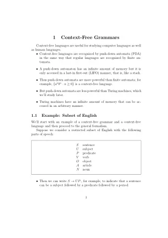
✬ ✩ Context-Free Grammars . . . were invented in the fifties, when Chomsky proposed different formalisms for describing natural language syntax. They were popularised by Naur with the Algol 60 report, and are often referred to as Backus-Naur Formalism (BNF). Standard tools for parsing owe much to this formalism, which indirectly has helped make parsing a routine task. It is extensively used to specify syntax of programming languages, and now also document formats (XML’s document-type definition). ✫ ✪ 6-1

✬ ✩ Context-Free Grammars (cont.) We have already used the formalism of context-free grammars. To specify the syntax of regular expressions we gave a grammar , much like → 0 R → 1 R → R ǫ → ∅ R → R ∪ R R → R ◦ R R → R ∗ R Hence a grammar is a set of substitution rules , or productions . We have the shorthand notation → 0 | 1 | ǫ | ∅ | R ∪ R | R ◦ R | R ∗ R ✫ ✪ 6-2

✬ ✩ Sentences A simpler example is this grammar G : → 0 A 1 1 A → A ǫ Using the two rules as a rewrite system, we get derivations such as ⇒ 0 A 11 A ⇒ 00 A 1111 ⇒ 000 A 111111 ⇒ 000111111 A is called a variable . Other symbols (here 0 and 1) are terminals . Compiler writers refer to a valid string of terminals (such as 000111111 ) as a sentence . The intermediate strings that mix variables and ✫ terminals are sentential forms . ✪ 6-3

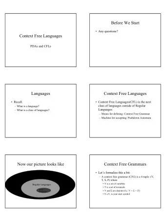
✬ ✩ Context-Free Languages Clearly a grammar determines a formal language. The language of G is written L ( G ). L ( G ) = { 0 n 1 2 n | n > 0 } A language which can be generated by some context-free grammar is a context-free language (CFL). It should be clear that some of the languages that we found not to be regular are context-free, for example { 0 n 1 n | n ≥ 1 } ✫ ✪ 6-4

✬ ✩ Context-Free Grammars Formally A context-free grammar (CFG) G is a 4-tuple ( V, Σ , R, S ), where 1. V is a finite set of variables , 2. Σ is a finite set of terminals , 3. R is a finite set of rules , each consisting of a variable (the left-hand side) and a sentential form (the right-hand side), 4. S is the start variable . The binary relation ⇒ on sentential forms is defined as follows. Let u , v , and w be sentential forms. Then uAw ⇒ uvw iff A → v is a rule in R . So ⇒ captures a single derivation step. ∗ Let ⇒ be the reflexive transitive closure of ⇒ . L ( G ) = { s ∈ Σ ∗ | S ∗ ⇒ s } ✫ ✪ 6-5

✬ ✩ Parse Trees Here is a grammar with three variables, 14 terminals, and 15 rules: → T | T + E E → F | F ∗ T T → 0 | 1 | . . . | 9 | ( E ) F When the start variable is unspecified, it is assumed to be the variable of the first rule. An example sentence in the language is (3 + 7) * 2 The grammar ensures that * binds tighter than + . ✫ ✪ 6-6

✬ ✩ Parse Trees (cont.) Here is a parse tree for (3 + 7) * 2 : E T F * T ( E ) F T + E 2 F T 3 F 7 ✫ ✪ 6-7

✬ ✩ Parse Trees (cont.) There are different derivations leading to the sentence (3 + 7) * 2 , all corresponding to the parse tree above. They differ in the order in which we choose to replace variables. Here is the leftmost derivation: E T ⇒ F ∗ T ⇒ ( E ) ∗ T ⇒ ( T + E ) ∗ T ⇒ ( F + E ) ∗ T ⇒ ( 3 + E ) ∗ T ⇒ ( 3 + T ) ∗ T ⇒ ( 3 + F ) ∗ T ⇒ ( 3 + 7 ) ∗ T ⇒ ( 3 + 7 ) ∗ F ⇒ ( 3 + 7 ) ∗ 2 ⇒ ✫ ✪ 6-8

✬ ✩ Ambiguity Consider the grammar → E + E | E ∗ E | ( E ) | 0 | 1 | . . . | 9 E This grammar allows not only different derivations, but different parse trees for 3 + 7 * 2 : E E E + E E * E 3 E * E E + E 2 7 2 3 7 ✫ ✪ 6-9

✬ ✩ Ambiguity (cont.) A grammar that has different parse trees for some sentence is ambiguous . Sometimes we can find a better grammar (as in our example) which is not ambiguous, and which generates the same language. However, this is not always possible: There are CFLs that are inherently ambiguous , for example, L = { a i b j c k | i = j or j = k } . (Consider parse trees for a 3 b 3 c 3 .) ✫ ✪ 6-10

✬ ✩ Chomsky Normal Form It is sometimes convenient to bring a CFG into a normal form. A simple normal form is Chomsky normal form where every rule is of one of these forms: → A B C → A a → S ǫ where S is the start variable, A may be the start variable, B and C are (non-start) variables, and a is a terminal. Theorem: Every CFL has a CFG in Chomsky normal form. ✫ ✪ 6-11

✬ ✩ Conversion to Chomsky Form The method for converting a grammar to Chomsky normal form is this: 1. Add a new start variable S 0 and rule S 0 → S . 2. Eliminate epsilon rules A → ǫ . 3. Eliminate unit rules A → B . 4. Eliminate useless symbols. 5. Ensure that right-hand sides with length greater than 1 consist of variables only. 6. Break right-hand sides of length 3 or more into several rules by introducing fresh variables. ✫ ✪ 6-12

✬ ✩ Eliminating Epsilon Rules If we have A → ǫ then we replace every occurrence of A on right-hand sides by ǫ . For example, → S 0 S → S 0 ǫ → S A S A B → S 0 S → S A A B → S A S A B → S S A B → S ǫ ⇒ → S A B → A ǫ → S A S B → B C → S S B → C a → S B → B C → C a A rule E → A gets replaced by E → ǫ unless we ✫ already removed that rule. A → ǫ is removed. ✪ 6-13

✬ ✩ Eliminating Unit Rules We replace a rule B → C by B → u for each rule C → u , unless B → u is a unit rule we already removed. → → (same as S ) S 0 S S 0 → → S 0 ǫ S 0 ǫ → → S A S A B S A S A B → → S A A B S A A B → → S S A B S S A B ⇒ → → S A B S A B → → S A S B S A S B → → S S B S S B → → S B S a → → B C B a → → C a C a ✫ ✪ 6-14

✬ ✩ Eliminating Useless Symbols There are two kinds of useless variables. First remove rules with a symbol such as A which is not generating : → S 0 S B → S 0 a → S 0 ǫ → S S B → S a → B a → C a ✫ ✪ 6-15

✬ ✩ Eliminating Useless Symbols (cont.) Then remove rules with a symbol such as C which is not reachable : → S 0 S B → S 0 a → S 0 ǫ → S S B → S a → B a This grammar is now in Chomsky normal form, but sometimes we need another two steps . . . ✫ ✪ 6-16

✬ ✩ Another Example Consider the grammar (with new start variable) → S E → T | T + E E → F | F ∗ T T → 0 | 1 | ( E ) F There are no epsilon rules, but several unit rules to eliminate: → 0 | 1 | ( E ) | F ∗ T | T + E S → 0 | 1 | ( E ) | F ∗ T | T + E E → 0 | 1 | ( E ) | F ∗ T T → 0 | 1 | ( E ) F ✫ ✪ 6-17

✬ ✩ Another Example (cont.) Now make right-hand sides of length more than 1 consist of variables: → 0 | 1 | L E R | F M T | T P E S → 0 | 1 | L E R | F M T | T P E E → 0 | 1 | L E R | F M T T → 0 | 1 | L E R F → L ( → R ) → ∗ M → + P ✫ ✪ 6-18

✬ ✩ Another Example (cont.) Finally cascade the rules as needed, introducing more variables: 0 | 1 | L ′ R | F ′ T | T ′ E → S 0 | 1 | L ′ R | F ′ T | T ′ E → E 0 | 1 | L ′ R | F ′ T → T 0 | 1 | L ′ R → F → ( L → ) R → ∗ M → + P L ′ → L E F ′ → F M → T ′ T P ✫ ✪ 6-19