CONTENTS OF DAY 2 I. Random Sampling 3 Connection with - PowerPoint PPT Presentation

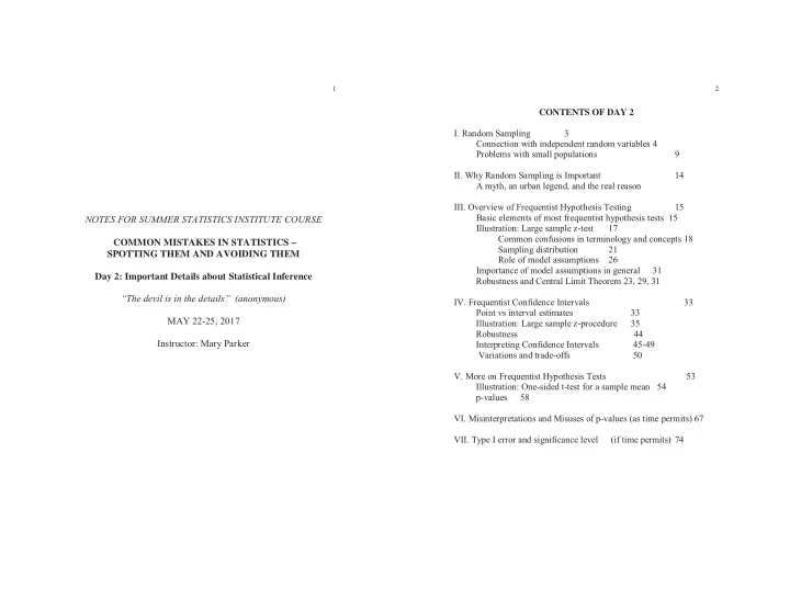
1 2 � CONTENTS OF DAY 2 I. Random Sampling 3 Connection with independent random variables 4 Problems with small populations 9 II. Why Random Sampling is Important 14 A myth, an urban legend, and the real reason III. Overview of Frequentist Hypothesis Testing 15 Basic elements of most frequentist hypothesis tests 15 NOTES FOR SUMMER STATISTICS INSTITUTE COURSE Illustration: Large sample z-test 17 Common confusions in terminology and concepts 18 COMMON MISTAKES IN STATISTICS – Sampling distribution 21 SPOTTING THEM AND AVOIDING THEM Role of model assumptions 26 Importance of model assumptions in general 31 Day 2: Important Details about Statistical Inference Robustness and Central Limit Theorem 23, 29, 31 “The devil is in the details” (anonymous) IV. Frequentist Confidence Intervals 33 Point vs interval estimates 33 MAY 22-25, 2017 Illustration: Large sample z-procedure 35 Robustness 44 Instructor: Mary Parker Interpreting Confidence Intervals 45-49 Variations and trade-offs 50 V. More on Frequentist Hypothesis Tests 53 Illustration: One-sided t-test for a sample mean 54 p-values 58 VI. Misinterpretations and Misuses of p-values (as time permits) 67 VII. Type I error and significance level (if time permits) 74

3 4 Distinctions and Notation: I. Random Sampling If we take a sample of units from the population , we have a In practice in applying statistical techniques, we’re interested in corresponding sample of values of the random variable . random variables defined on the population under study. In Example 1: Recall the examples mentioned yesterday: � The random variable is “difference in blood pressure with and without taking the drug.” 1. In a medical study, the population might be all adults over age 50 who have high blood pressure. o Call this random variable Y (upper case Y) 2. In another study, the population might be all hospitals in the U.S. that perform heart bypass surgery. � The sample of units from the population is a sample of adults 3. If we’re studying whether a certain die is fair or weighted, the population is all possible tosses of the die. over age 50 who have high blood pressure. In these examples, we might be interested in the following random o Call them person 1, person 2, etc. variables: � The corresponding sample of values of the random variable Example 1: The difference in blood pressure with and without will consist of values we will call y 1 , y 2 , ..., y n (lower case taking a certain drug. y’s), where Example 2: The number of heart bypass surgeries performed in a particular year, or the number of such surgeries that are o n = number of people in the sample; successful, or the number in which the patient has o y 1 = the difference in blood pressures (that is, the value complications of surgery, etc. of Y) for the first person in the sample; Example 3: The number that comes up on the die. o y 2 = the difference in blood pressures (that is, the value of Y) for the second person in the sample; o etc.

5 6 We can look at this another way , in terms of n random variables Different types of random sampling Y 1 , Y 2 , ..., Y n , described as follows: Some of the main types of random (probability-based) sampling that we can use are the following. � The random process for Y 1 is “pick the first person in the ( While not a comprehensive list, this is enough to illustrate the sample”; the value of Y 1 is the value of Y for that person – differences and their effect on the analyses.) i.e., y 1 . 1. Simple random sample from a finite population without � The random process for Y 2 is “pick the second person in the replacement. sample”; the value of Y 2 is the value of Y for that person – ( What we usually are thinking about .) i.e., y 2 . 2. Simple random sample from a finite population with � etc. replacement. ( How strange! Why would anyone want to do that ?) The difference between using the small y's and the large Y's is that when we use the small y's, those are actual values we found, 3. Simple random sample from an infinite population where, with the large Y’s we are still thinking of them as random ( Tossing a die six times, etc .) variables which will change when we choose a different sample from the same population by the same probability-based (random) 4. Stratified random sample from a finite population process. ( Divide the population into strata, such as in Example 2, teaching hospitals and non-teaching hospitals. Take a simple Note : Because the Y i ’s are random variables, each has a random sample from each stratum, and combine those into one distribution. Whether they are considered to have exactly the sample from the population.) same distribution or “almost the same” distribution, is the topic of the next few slides. Now, back to the mathematics . . . The easiest processes to analyze mathematically are those in which the individual random variables Y 1 , Y 2 , ... , Y n are independent. Intuitively speaking, " independent " means that the values of any subset of the random variables Y 1 , Y 2 , ... , Y n do not influence the probabilities of the values of the other random variables in the list .

7 8 Note : Because the Y i ’s are random variables, each has a 3. Simple random sample from an infinite population distribution. It would also be convenient, mathematically, if those random variables had the same probability distribution, which we What, exactly does an infinite population mean? call identically distributed (in this example, the distribution of Y). That means that our random variables Y i are values from a particular probability distribution. So when we take a value for Y 1 from that population, we next take the value Y 2 from So, in which of our four types of random samples are the Y i ’s the same population. So here the Y i values are independent independent and identically distributed (denoted iid) ? and identically distributed. (Tossing a fair die: the population has a discrete uniform 1. Simple random sampling without replacement. Not here. distribution on the set of whole numbers from 1 to 6.) Suppose the population has 1000 members in it. When we choose the value for Y 1 then there are 999 members left in 4. Stratified random sampling. the population from which we will choose Y 2. Considering this gives us no new insights into this situation So we are not choosing Y 2 from exactly the same population about independent and identically distributed random as we chose Y 1 . We can also see that Y 2 is not independent variables Y i , so we will postpone discussion of it for now. of Y 1 because knowing the value for Y 1 gives us some information about the value for Y 2 . 2. Simple random sampling with replacement. YES, these are iid. Suppose the population has 1000 members in it. We choose the value for Y 1 , record that value as y 1 , and then replace that value in the population before we draw a value for Y 2 . So we are drawing Y 2 from the same population we drew Y 1 from, and the value we chose for Y 1 has no impact on the value we chose for Y 2 . Let’s pause here. Now we see why someone might choose to do this strange method of sampling with replacement. It makes the mathematics easier!

9 10 What mathematics? Which of our applied examples are iid? Recall Example 3 above : We toss a die; the number that comes up The corrections needed to the usual formulas are multipliers on the die is the value of our random variable Y. to lower the variance appropriately. � In terms of the preliminary definition: For single means and single proportions, they are something n � 1 o The population is all possible tosses of the die. like N where n is the sample size and N is the population size. o A simple random sample is n different tosses. � The different tosses of the die are independent events (i.e., Try for yourself to see how large a fraction of the population what happens in some tosses has no influence on the other you need to sample to get enough reduction in the variance tosses), which means that in the precise definition above, the when estimating a single mean or single proportion to be random variables Y 1 , Y 2 , ... , Y n are indeed independent: The worth correcting. numbers that come up in some tosses in no way influence the numbers that come up in other tosses. More explanation of this is available at https://www.ma.utexas.edu/users/parker/sampling/repl.htm Recall Examples 1 and 2 above: Example 1: Choose a random sample of adults over 50 with high blood pressure. How to avoid mistakes when sampling without replacement and using the standard formulas in applied statistics courses. Example 2: Choose a sample of hospitals in the US that Pay attention to what percentage of the population you are perform heart bypass surgery. sampling. If it is a small percentage, don’t worry about it. No one explicitly said whether the sampling would be with If it is a larger percentage (more than 5% or 10%) then replacement or without replacement, but we suspect that those congratulate yourself on getting quite a lot of information doing the sampling would do it without replacement. But we just about your population! And then find the finite correction learned that the mathematics is a lot easier if we sample with factors needed to adjust your variances to “get credit in your replacement. What happens? Is this a major problem? calculations” for the extra information you have! Mathematics can come to the rescue!