Global Illumination Multi-Sampling Path Tracing Simple Sampling - - PowerPoint PPT Presentation

Global Illumination

Multi-Sampling Path Tracing

Simple Sampling

• Josef talked about all of the details

behind signals and sampling

• For assignment purposes, things will be

a bit simpler…

Sampling techniques

• Uniform
• Random

– We will focus on this one today

• Jittered

– This is not much harder than the above (extra credit)

Random Sampling

• You will find that it actually works well

enough a lot of the time

• Pick a random point within the area

being sampled

• Let’s start by sampling in pixels

2x2 Image

for each pixel (i, j) x = 2.0f * (j - xres/2.f + 0.5f)/xres; y = 2.0f * (i - yres/2.f + 0.5f)/yres;

• 1

1 1

[-.5, -.5] [.5, -.5] [-.5, .5] [.5, .5]

Everything in the range of x = [-1 .. 0], y = [-1 .. 0] falls within the same pixel

Sampling a Pixel

Randomly offset (x, y) within the area of the pixel Take as many samples as desired How do we offset?

• 1

1 1

[-.5, -.5] [.5, -.5] [-.5, .5] [.5, .5]

In General

x – 1/width, y – 1/height

[x, y]

x + 1/width, y – 1/height x – 1/width, y + 1/height x + 1/width, y + 1/height

inv_width = loadf(0, 2) inv_height = loadf(0, 5)

Random Point in Pixel

// value between -1 .. 1 x_off = (trax_rand() - .5f) * 2.f y_off = (trax_rand() - .5f) * 2.f x_off *= inv_width y_off *= inv_height x += x_off y += y_off camera.makeRay(ray, x, y);

[x, y]

inv_width

Filtering

• Box

– We will focus on this one today

• Triangle

– More difficult than the above, but not terribly (requires samples outside pixel)

• Gaussian

– Same infrastructure as triangle filter, different math

Box Filter

• Simply means all samples are weighted

equally

• For each sample, add ray contribution

to the color of the pixel

– Pixel will likely end up with > 1 intensity

• Then divide color by num_samples

– then clamp to 0 .. 1

Putting it all together

for(pixels) for(num_samples)

• camera.makeRay(ray, x, y) // x and y
• have been
• randomly
• permuted
• bvh.intersect(hit, ray)
• result += shade(...) // +=, not =

result /= num_samples // box filter image.set(i, j, result);

Global Illumination

• So far, we have looked at light from

specific sources

– Light source – Reflections – Refractions

• In reality, it isn’t this simply

– Still using “ambient” term for everything not in direct light

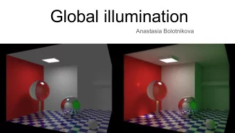
Global Illumination

Global Illumination

Global Illumination

• Metropolis
• Ambient Occlusion
• Photon Mapping
• Path Tracing

– arguably the most straight-forward

• Others…

Path Tracing

• Pure path tracing is the most naïve

solution to global illumination

– Also the most elegant (my opinion)

• Path tracing for Lambertian shading
• 1. Cast a ray from the camera
• 2. Multiply attenuation by material
• From that point, cast exactly 1 ray in a random

direction

• 3. Repeat step 2 until light source is hit
• 4. Final color = attenuation * emitted light

Path Tracing

Random reflection direction

N

• Pick a random direction on the normal hemisphere
• How?

Orthonormal basis

• First, we need to find a set of
• rthogonormal axes based on the

normal

– This will be sort of like a “camera”

• Set the Z axis in our new basis equal to

the normal

– Find any X and Y orthogonal to Z and unit length (“orthonormal”) – How?

Orthonormal basis

• Remember, cross product returns a vector

that is perpendicular to both input vectors Vector Z = normal; cross(N, any vector) Pick one of (1, 0, 0), (0, 1, 0), (0, 0, 1)

• This result will be perpendicular to the normal

– But what if the vector we pick is parallel to the normal? – Result will be zero vector

Orthonormal basis

• Choose axis with smallest component in

normal

if(N.x < N.y && N.x < N.z) { axis = vec(1.0f, 0.0f, 0.0f); } else if (N.y < N.z) { axis = vec(0.0f, 1.0f, 0.0f); } else { axis = vec(0.0f, 0.0f, 1.0f); }

Orthonormal basis

• Last axis is cross product of other two

X = normal.cross(axis).normalize() Y = normal.cross(X)

• Now we have a new axis system

– X and Y are tangent to the surface – Z is normal to the surface

Orthonormal basis

Z X

Y not drawn in 2D example

Hemisphere sampling

• Pick a random vector on the unit hemisphere

defined by our new basis

• Option 1:

– Define the “hemicube” (half cube) on the surface – Randomly pick points inside the cube until we get

• ne that is inside the hemisphere

– Will be uniformly distributed (actually a bad thing)

• Option 2:

– Randomly pick points on the unit disc – Project out to hemisphere – Not uniformly distributed (more later)

Hemisphere sampling

• Pick random point inside the unit disc:

do { u = trax_rand() v = trax_rand() u *= 2.0f; u -= 1.0f; v *= 2.0f; v -= 1.0f; u_2 = u * u; v_2 = v * v; } while((u_2 + v_2) >= 1.0f);

Path Tracing

• We now have a vector (u, v) on the (X, Y)

plane

• Need to project up Z axis to make unit length

(this will be a point on unit hemisphere)

• We know length needs to be 1.0
• w = sqrt(1 – u2 – v2)
• refDir = (X * u) + (Y * v) + (normal * w)

Cosine weighting

• This generates samples weighted more

heavily towards the normal

• Specifically, weighted by the cosine of the

angle between the reflected ray and the normal

• Lambertian shading says we should multiply

incoming light by cosine of angle

– With samples cosine-weighted, we don’t need to

Path Tracing

Path Tracing

• Obviously we need more than 1 sample per

pixel

• With more samples, the image begins to

converge to the “correct” result

– In practice, requires more than is reasonable – Unless you have hours, even days to wait

100 samples per pixel

100k spp, tone mapped

Sampling

• Two techniques:
• 1. Take multiple GI samples per hit point
• 2. Take 1 GI sample per hit point, increase

samples per pixel

• Option 2 will provide anti-aliasing at the same

time

– But we also may not need that many primary ray samples

• Option 1 muddies implementation a bit

Path Length

• In an enclosed space, a path may bounce

forever

• Need some way of terminating “useless”

paths – Russian roulette – Max depth – Min attenuation

Attenuation

• Every time a ray bounces, it is attenuated by

that material (loses energy)

• Start with attenuation (color) of (1, 1, 1),

multiply it by color of hit material on each bounce

• If total energy becomes less than small

amount, kill the path

Importance sampling

• Probabilistically, most paths of light will not hit

a light source

• These paths don’t contribute anything to the

image, and are wasted work

• With point light sources, no light will be found

whatsoever

• Kajia path tracing combines pure path tracing

with direct Lambertian shading

Kajia path tracing

... for each sample attenuation = Color(1.f, 1.f, 1.f) Ray r = cameraRay(…) while(depth < max_depth) {

• HitRecord hit
• bvh.intersect(hit, ray)
• result += shade(…) * attenuation
• attenuation *= mat_color
• r = hemiRay(…)
• depth++

}

Kajia path tracing

• The previous pseudo code doesn’t stop when

hitting a light

• In TRaX, we will never hit the light (point

lights only)

– Pure path tracing won’t work with point lights

• Must not be recursive!

Kajia path tracing

• Kajia path tracing samples a random light

source directly (not all of them)

– We only have one anyway

• Sampling light sources directly does not

account for visible intensity of light

– May be obscured slightly – May be far away – Can’t handle transparent materials

Pure Path Tracing

• Automatically solves various problems

– Caustics – Visible intensity of light sources

• Simplifies architecture

– No longer need “Light” objects (use emissive term in material)

• Requires bajillions of samples to converge

– Probability of path hitting a light source is low

Pure Path Tracing

Total energy in the scene will be low – based on probability of hitting a light… Need some kind of tone mapping to bring things in to reasonable range

Tone-Mapped

Exact same information as previous image

Free caustics