Congestion Pricing Modeling and Prepared for Southern Results for - PowerPoint PPT Presentation
Congestion Pricing Modeling and Prepared for Southern Results for xpress Travel Choices Study Results for Express Travel Choices Study California Association of Kazem Oryani and Cissy Kulakowski, CDM Smith Governments (SCAG) Portland, Oregon,
Congestion Pricing Modeling and Prepared for Southern Results for xpress Travel Choices Study Results for Express Travel Choices Study California Association of Kazem Oryani and Cissy Kulakowski, CDM Smith Governments (SCAG) Portland, Oregon, October 22 ‐ 25, 2013 2013 2013 Association of Metropolitan Planning Organization (AMPO) Annual Conference 1
Objective To estimate revenue potentials and network p performance measures for range of pricing scenarios as an input for policy discussion and selection for pre ‐ implementation analysis. 2
Southern California Association of Governments (SCAG) ( ) • Year 2010 Population ‐ 18 Million • SCAG Region is Home to 49 Percent of California Population • Year 2035 Population ‐ 22 Million San Bernardino Co. • Increase of 4 Million Increase of 4 Million Ventura Los Co. Angeles Population in 25 Years Co. or 160,000 Person Per Riverside Year (Each Year, One Year (Each Year, One Orange Co. Co Co. Small City Added) Imperial Co. 3
Year 2035 Traffic • System – Vehicle trips ‐ 48.8 million – Average speed (mph) ‐ 34.7 – Average trip length (miles) ‐ 12.1 Average trip length (miles) 12 1 – Average trip time (min) ‐ 20.9 • Freeways – Vehicle trips ‐ 29.7 million – Average speed (mph) ‐ 43.9 – Average trip length (miles) ‐ 10.9 A i l h ( il ) 10 9 – Average trip time (min) ‐ 14.9 4
Inter ‐ County Person Trip Flows Weekday Work 5
Inter ‐ County Person Trip Flows Weekday Non ‐ Work 6
Inter ‐ County Person Trip Flows Weekday Total 7
New Model Components • Changes in Time ‐ of ‐ day Travel Changes in Time of day Travel Due to Pricing • Trip Suppression Due to Pricing • Route Choice Due to Pricing 8
Model System Structure Original SCAG SCAG Model Enhanced Model For Pricing Analysis Trip Trip Trip Trip Generation Generation Trip Destination Distribution Choice Enhancements Mode By CDM Smith Choice Mode Mode Choice Choice Choice Enhancements E h By PB Enhanced Time ‐ of ‐ day Time ‐ of ‐ Day Trip Trip Suppression Trip Enhanced Trip Assignment Assignment (Route Choice) (Route Choice) 9
Tools and Databases • Existing Time ‐ Period Model – AM peak (6am ‐ 9am) – MD (9am ‐ 3pm) – PM peak (3pm ‐ 7pm) PM k (3 7 ) – Night (7pm ‐ 6am) – 4 periods p • Enhanced Model: – 30 (½ hour periods) (6am ‐ 9pm) – 1 night period (9pm ‐ 6am) – 31 periods 10
Model Estimation • Trip suppression / time ‐ of ‐ day changes based on Stated Preference Survey: Preference Survey: – More than 3,600 samples • Coverage (Six county SCAG Region): Coverage (Six county SCAG Region): – Imperial, Los Angeles, Orange, Riverside, San Bernardino, and Ventura Counties. 11
Model Estimation Time ‐ of ‐ Day Model Estimation Based on More Time of Day Model Estimation Based on More Than 16,000 SCAG Household Travel Surveys in 2001 Including More Than 88,000 Full Person Trip Records. 12
Year 2010 Stated Preference Survey • Stated Preference Survey to Support Model Changes – 3,600 survey record for all six SCAG counties – Discrete choice model by trip purpose: work business trips, non ‐ work – Time ‐ of ‐ day: peak, off ‐ peak $2 00 $2.00 $3 00 $3.00 $4 00 $4.00 $3.00 $3 00 $2 00 $2.00 10,000 9,000 8,000 7,000 Hourly Traffic 6,000 5,000 4,000 H 3,000 2,000 1,000 0 0 5:00 6:00 7:00 8:00 9:00 10:00 Hour 13
Hypothetical Reaction to Pricing for Range of Fees 100% 7% 4% 5% 8% 10% 4% 12% 5% 15% 6% 17% 90% 90% 20% 20% 7% 7% 23% 23% 8% 14% 13% 9% 13% 80% 9% 12% 10% 11% 7% 11% 11% 8% 8% 10% 12% 70% 8% 10% 7% 9% 7% 9% 8% 9% 9% 9% Percent Share e 60% 60% 8% 8% 8% 8% 9% 8% 9% 8% 9% 10% 50% 9% 9% 9% 40% 64% 64% 62% 62% 30% 60% 57% 54% 51% 48% 45% 42% 20% 38% 10% 0% $1 $2 $3 $4 $5 $6 $7 $8 $9 $10 Area Pricing Fee Current Destination Peak Current Destination Shift Early Current Destination Shift Late Current Destination Shift Late Current Destination HOV Current Destination HOV Alternate Destination Transit 14
Variables Used in Model Estimation • Used Multinomial Logit Formulation for Time of day Model Time ‐ of ‐ day Model • Logit Based Toll Diversion Model for Trip Assignment • Utilized Enhanced Model for Scenario Analysis 15
Variables Used in Model Estimation • Departure Time • Arrival Time • Origin Zone • Destination Zone Destination Zone • Trip Purpose • Mode • Traveler’s Household Size • Traveler s Household Size • Traveler’s Household Income • The Number of Household Workers • The Number of Household Vehicles • The Number of Household Vehicles • Traveler’s Age • Traveler’s Employment Industry Type 16
HBWD From Home Trip Time ‐ of ‐ Day Choice Model Summary Variables in Utility Functions Alternatives Shift Delay Delay Distance Distance Drive Constant Delay Distance Inc_H Inc_M_H Inc_M_L HH_Size Age Pop_O Shift Shift^2 Shift Shift^2 Alone AM1 1.5 3.579 (7.647) 0.014 0.011 AM2 AM2 1 1 4 094 (8 770) 4.094 (8.770) (2.626) (3.279) -0.032 -0.014 AM3 0.5 4.409 (9.447) 0.917 0.480 0.236 -0.257 -0.008 0.215 -0.003 (-5.342) (-3.600) AM4 0 4.495 (9.624) (8.559) (5.948) (2.787) (-11.041) (-2.697) (2.125) (-1.397) 0.037 0.030 -0.007 AM5 0.5 4.056 (8.661) (1.579) (-1.303) (-1.009) AM6 1 3.858 (8.217) MD1 3 3.413 (7.085) MD2 2.5 3.047 (6.305) MD3 2 2.408 (4.935) ( ) MD4 1.5 2.328 (4.763) MD5 1 2.195 (4.476) -0.010 -0.024 0.485 -0.197 -0.011 0.415 -0.006 MD6 0.5 2.108 (4.289) MD7 0 1.858 (3.753) (Constrained) (-7.908) (4.842) (-7.054) (-3.437) (3.292) (-1.874) MD8 0.5 2.580 (5.300) MD9 1 2.445 (4.997) -0.012 MD10 1.5 2.617 (5.352) (-3.524) MD11 2 2.597 (5.287) MD12 2.5 2.472 (4.997) PM1 3 2.469 (5.975) PM2 2.5 2.324 (5.674) -0.003 PM3 2 2.015 (4.883) (-1.476) PM4 1.5 2.158 (5.301) PM5 1 1.908 (4.623) PM6 0.5 1.868 (4.515) -0.028 -0.012 -0.107 -0.025 0.429 -0.004 PM7 PM7 0 0 1.598 (3.783) 1 598 (3 783) (-2 400) ( 2.400) (-1 936) ( 1.936) (-2 841) ( 2.841) (-5 192) ( 5.192) (2 425) (2.425) ( 1.016) (-1 016) PM8 0.5 1.747 (3.981) PM9 1 1.517 (3.302) -0.052 0.025 PM10 1.5 0.973 (2.015) (-2.048) (2.408) PM11 2 0.718 (1.543) PM12 2.5 0.000 NT 0 3.725 (7.720) Note: Value in parentheses is the t-statistics. Note: Value in parentheses is the t statistics. Observations: 7,368 Final Log Likelihood: -19,733 ρ 2 w.r.t. 0: 0.22 17
Change in Tripmaking (Trip Suppression / Inducement) Peak Non work Trip Peak Non ‐ work Trip Travel Time Difference Toll Difference Difference 0 ‐ 5 ‐ 10 ‐ 15 ‐ 20 $0.00 +0.0% +1.2% +2.4% +3.6% +4.7% $2.00 ‐ 3.8% ‐ 2.6% ‐ 1.5% ‐ 0.3% +0.9% $4.00 ‐ 7.6% ‐ 6.5% ‐ 5.3% ‐ 4.1% ‐ 2.9% $6.00 ‐ 11.5% ‐ 10.3% ‐ 9.1% ‐ 7.9% ‐ 6.7% $8.00 ‐ 15.3% ‐ 14.1% ‐ 12.9% ‐ 11.7% ‐ 10.6% $10.00 $10 00 ‐ 19.1% 19 1% ‐ 17.9% 17 9% ‐ 16.7% 16 7% ‐ 15.6% 15 6% ‐ 14.4% 14 4% (Negative = Suppression, Positive = Inducement) 18
Trip Suppression Model The models were developed from regression analysis on the responses to the trip suppression question in the survey developed by comparing the change in trips pp q y p y p g g p made against the change in utility of each trip. The generic trip regression equation is shown as: Cost after after * * cos t LN ( income / ) Tr m * LN ( d 1 ) Where: • Δ Tr is the percentage difference in the number of trips • m is the regression coefficient • LN(d+1) is the natural log of trip distance in miles plus 1 • Β cost is the toll cost coefficient • Cost after is the toll cost with pricing • Income/ λ is the median household income divided by λ 19
Base Case Performance Measures (000’s) AM PM Total System Peak Midday Peak Evening Night Total Vehicle Trips 9,730 18,054 14,440 3,040 3,542 48,805 VMT 121,398 187,119 179,554 36,071 65,166 589,308 VHT 4,163 4,513 6,367 746 1,214 17,003 Average Speed (mph) 29.2 41.5 28.2 48.4 53.7 34.7 Average Trip Length (miles) 12.5 10.4 12.4 11.9 18.4 12.1 Average Trip Time (min) 25.7 15.0 26.5 14.7 20.6 20.9 AM PM All F All Freeways P Peak k Midd Midday Peak P k E Evening i Night Ni ht T t l Total Vehicle Trips 6,126 9,699 8,616 2,069 3,180 29,691 VMT 62,476 103,845 90,831 21,793 44,739 323,684 VHT 1,740 1,839 2,832 323 643 7,378 Average Speed (mph) 35.9 56.5 32.1 67.4 69.6 43.9 Average Trip Length on Fwy (miles) Average Trip Length on Fwy. (miles) 10.2 10 2 10.7 10 7 10.5 10 5 10 5 10.5 14 1 14.1 10.9 10 9 Average Trip Time on Fwy. (min) 17.0 11.4 19.7 9.4 12.1 14.9 AM PM All Other Roads Peak Midday Peak Evening Night Total VMT 58,922 83,274 88,722 14,278 20,427 265,623 VHT VHT 2 422 2,422 2 675 2,675 3,535 3 535 422 422 571 571 9,626 9 626 Average Speed (mph) 24.3 31.1 25.1 33.8 35.8 27.6 AM PM Peak Midday Peak Evening Night Total Vehicle Trips Crossing 455 682 558 125 242 2,062 Downtown Cordon 20
Scenarios Examined Base Case Regional Freeway System Regional Freeway System 21
Scenarios Examined (cont’d) 1 ‐ Strategic Express Lanes Network: HOV3+Free 2 ‐ Strategic Express Lanes Network: HOV2+Free Strategic Express Lane Network Strategic Express Lane Network 22
Recommend
More recommend
Explore More Topics
Stay informed with curated content and fresh updates.
