Internet congestion control: TCP Internet congestion control: TCP - PowerPoint PPT Presentation
Internet congestion control: TCP Internet congestion control: TCP 1988: "Congestion Avoidance and Control" (Jacobson/Karels) Combined congestion/flow control for TCP Goal: stability - in equilibrum, no packet is sent into the
Internet congestion control: TCP Internet congestion control: TCP • 1988: "Congestion Avoidance and Control" (Jacobson/Karels) Combined congestion/flow control for TCP • Goal: stability - in equilibrum, no packet is sent into the network until an old packet leaves – ack clocking, “conservation of packets“ principle – possible through window based stop&go - behaviour • Superposition of stable systems = stable -> network based on TCP with congestion control = stable • Today, TCP dominates the Internet (WWW, ..) recent backbone measurement: 98% TCP traffic
AIMD Background AIMD Background MIMD MIMD Fairness Fairness Line Line AIAD AIAD User 2 Allocation x2 User 2 Allocation x2 AIMD AIMD Overload Overload Starting Starting Point Point Desirable Desirable Starting Starting Efficiency Efficiency Point Point Line Line Underload Underload User 1 Allocation x1 User 1 Allocation x1
Some reasons for TCP stability Some reasons for TCP stability • Exponential backoff: “For a transport endpoint embedded in a network of unknown topology and with an unknown, unknowable and constantly changing population of competing conversations, only one scheme has any hope of working - exponential backoff - but a proof of this is beyond the scope of this paper.“ • Conservation of packets: “The physics of flow predicts that systems with this property should be robust in the face of congestion.“ • Additive Increase, Multiplicative Decrease: Not explicitely cited as a stability reason in the paper ! – ...but in 1000‘s of other papers!
“Proofs“ of TCP stability “Proofs“ of TCP stability • AIMD: Chiu/Jain: diagram + algebraic proof homogeneous RTT case • steady-state TCP model: window size ~ 1.22/sqrt(p) (p = packet loss) • Johari/Tan, Massoulié, ..: – local stability, neglect details of TCP behaviour (fluid flow model, ..) – assumption: “queueing delays will eventually become small relative to propagation delays“ • Steven Low: – Duality model (based on utility function / F. Kelly, ..): Stability depends on delay, capacity, load and AQM !
Extended Use of Vector Diagrams Extended Use of Vector Diagrams • Problem: – Stability analysis very complex – TCP-like mechanism design difficult • Solution: – Extended use of vector diagrams! • Analyze actual results (from simulation or real life measurements) • Instead of just explaining a concept, design in the diagram space – Necessary simplifications may even be less dramatic!
How Stable is AIMD / async. RTT? How Stable is AIMD / async. RTT? U 2 SER 1.0000 0.9500 0.9000 • Simple simulation 0.8500 (no queues, ..) 0.8000 • RTT: 7 vs. 2 0.7500 • AI=0.1, MD=0.5 0.7000 0.6500 • Simul. time=175 0.6000 0.5500 0.5000 0.4500 0.4000 0.3500 0.3000 0.2500 0.2000 0.1500 0.1000 0.0500 0.0000 -0.0500 1.0000 User 1 0.0000 0.2000 0.4000 0.6000 0.8000
How is AIMD distorted in TCP? How is AIMD distorted in TCP? TCP 2 10.0000 9.5000 • ns-2 simulator 9.0000 • TCP Tahoe 8.5000 • equal RTT 8.0000 7.5000 • 1 bottleneck link 7.0000 6.5000 6.0000 5.5000 5.0000 4.5000 4.0000 3.5000 3.0000 2.5000 2.0000 1.5000 1.0000 TCP 1 2.0000 4.0000 6.0000 8.0000 10.0000 12.0000 14.0000
Problems with TCP Problems with TCP • TCP over wireless: checksum error -> packet drop misinterpretation • TCP over “long fat pipes“: large bandwidth*delay product – long time to reach equilibrium, MD = dramatic! • TCP reaches equilibrium, but not a stable point – fluctuations lead to regular packet drops & reduced throughput – fluctuations not feasible for streaming multimedia apps • TCP Vegas: interpret delay as congestion ... but: similar delay, different available bandwidth!
Enhancement idea: ATM ABR Enhancement idea: ATM ABR • TCP -> TCP/RED -> TCP/RED/ECN -> TCP/RED/Multilevel ECN -> ... True for all • logical consequence: „ECN“ with fine granularity mechanisms which use binary (explicitely ask for congestion information) feedback! • Routers know more about congestion. TCP-AI is like guessing and reacting when it is already too late. • Idea related to ATM Available Bit Rate (ABR) service: – Resource management (RM) cells query the network for ECN flag & Explicit Rate information Often: – framework for sophisticated ER calculations Fairness through -> 1000s of papers flow counting -> not scalable!
PTP: The Performance Transparency PTP: The Performance Transparency Protocol (draft- -welzl welzl- -ptp ptp- -05.txt) 05.txt) Protocol (draft • “Generic“ ECN / BECN - to carry traffic information (e.g. queue length, ..) • Stateless & simple -> scalable! No problems w/ • Only every 2nd router needed for full functionality wireless links – If less routers support it, results are an upper limit unless combined with packet loss! • Available Bandwidth Determination: – nominal bandwidth (“ifSpeed“) + 2* (address + traffic counter (“if(In/Out)Octets“) + timestamp) = available bandwidth • two modes: “forward packet stamping“ / “direct reply“ (not for available bandwidth (byte counters))
PTP: How does it work? PTP: How does it work? • Forward packet stamping: Router 3 1 2 Sender Receiver B-?-c S-a A-b C-r 9>8! 7=7 6>5! Upper case: outgoing interface "Init 9" Lower case: TTL: 8 TTL: 7 TTL: 6 TTL: 4 9-4-5=0, incoming interface complete TTL-C: 9 TTL-C: 7 TTL-C: 6 TTL-C: 4 Bwinfo Request: a BWinfo a BWinfo a BWinfo Bwinfo A Bwinfo A BWinfo A BWinfo table B Bwinfo B BWinfo c BWinfo C Bwinfo – The receiver can tell if the information is complete (DS Count, TTL)
PTP: How does it work? /2 PTP: How does it work? /2 • Direct reply: – Routers compare values; if requirements cannot be met... • the values are updated, the packet is redirected to the sender – Similar to RSVP reservation setup – Does not work with available bandwidth (traffic counter) – Advantageous for satellite links! • Forward packet stamping satellite usage scenario: 1st ground station acts as a receiver - only relies on PTP
Design algorithm Design algorithm • find useful (closely related) ATM ABR mechanism • start with simplifications, then expand the model • A new mechanism must work for 2 users, equal RTT – simple analysis similar to Chiu/Jain (diagram + math) • it must also work for heterogeneous RTTs – simulate using a simple diagram based simulator – analyze using extended vector diagram analysis • it must also work for more users and more realistic scenarios – simulate with ns
The ATM ABR best match: CAPC The ATM ABR best match: CAPC • “Congestion Avoidance with Proportional Control“ (A. Barnhart 1994) • Uses load factor LF: Input Rate IR / Target Rate R0 – R0 e.g. 95% of nominal bandwidth, d = 1 - LF (available bandwidth) • “As long as the incoming rate is greater than R0, the desired rate, ERS will diminish at a rate that is proportional to the amount by which R0 is exceeded. Conversely, whenever the incoming rate is less than R0, ERS will increase.“ • for each new cell entering the queue: LF<=1: ERX = min(ERU, 1 + d*Rup) ... else ERX = max(ERF, 1 + d*Rdn) ERS = ERS*ERX • constants: Rup, Rdn define the speed of rate increase / decrease, ERU, ERF = upper / lower bound • different default values for LAN and WAN! hint for RTT dependance!
Conversion for packet nets: CADPC Conversion for packet nets: CADPC • “Congestion Avoidance with Distributed Proportional Control“ • Only ask for current load, do calculations at sender • Fairness: sender 1 RTT = x * sender 2 RTT – sender 1 needs to calculate ERS x times -> ERS = ERS*(ERX^x) • Result in Chiu-Jain-diagram-simulator: Note: multiplicative! – max-min fairness approximated for limited rtt variations (trade-off between Rup, Rdn and allowed RTT‘s) – not good enough, but gives a hint that weighing the rate changes with the user‘s properties can lead to max-min fairness!
CADPC Design CADPC Design • Idea: – relate user‘s current rate to the state of the system! (also in LDA+) Thought: in the Chiu-Jain-diagram, if the rate increase is indirectly proportional to the user‘s current rate, the rates will equalize. • erx = 1 + rup * (1.0 - myRate/traffic) does not work! e.g. synchronous case -> myRate/traffic = constant! • Solution: – erx = 1 + rup * (1.0 - myRate/d) relationship between user‘s rate and available rate keeps changing! • Enhancement: – dependence on rup not desirable; rate changes should be proportional to the current load -> use d instead of rup!
CADPC vector diagram analysis CADPC vector diagram analysis
CADPC synchronous case analysis CADPC synchronous case analysis • Final formula per user: d = traffic / r0; erx = 1 + d * (1.0 - myRate/d); ers = ers*erx; (Special form of) • Combined: logistic equation x ( t ) x i (t) = rate => stable! + = + − x ( t 1 ) x ( t ) 1 d 1 i i i n of user i, ∑ x ( t ) j n users = − j 1 1 r 0 • after some straight- n ∑ + = + − − x ( t 1 ) x ( t ) r 1 r x ( t ) x ( t ) forward derivations: i i 0 0 i j = j 1
Recommend


More recommend
Explore More Topics
Stay informed with curated content and fresh updates.