Configurational-Bias Monte Carlo N interacting particles in volume V - PowerPoint PPT Presentation
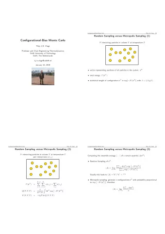
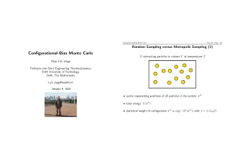
Configurational-Bias Monte Carlo Thijs J.H. Vlugt [1] Random Sampling versus Metropolis Sampling (1) Configurational-Bias Monte Carlo N interacting particles in volume V at temperature T Thijs J.H. Vlugt Professor and Chair Engineering
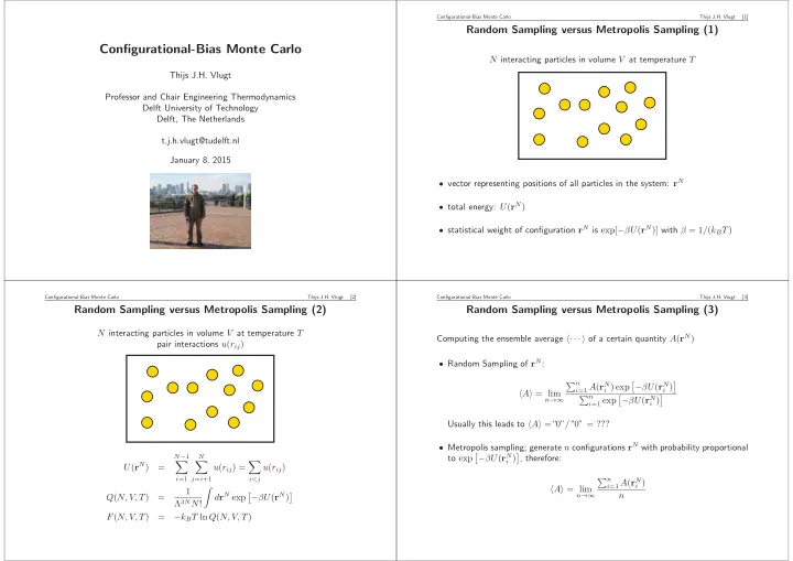
Configurational-Bias Monte Carlo Thijs J.H. Vlugt [1] Random Sampling versus Metropolis Sampling (1) Configurational-Bias Monte Carlo N interacting particles in volume V at temperature T Thijs J.H. Vlugt Professor and Chair Engineering Thermodynamics Delft University of Technology Delft, The Netherlands t.j.h.vlugt@tudelft.nl January 8, 2015 • vector representing positions of all particles in the system: r N • total energy: U ( r N ) • statistical weight of configuration r N is exp[ − βU ( r N )] with β = 1 / ( k B T ) Configurational-Bias Monte Carlo Thijs J.H. Vlugt [2] Configurational-Bias Monte Carlo Thijs J.H. Vlugt [3] Random Sampling versus Metropolis Sampling (2) Random Sampling versus Metropolis Sampling (3) N interacting particles in volume V at temperature T Computing the ensemble average �· · · � of a certain quantity A ( r N ) pair interactions u ( r ij ) • Random Sampling of r N : � n i =1 A ( r N − βU ( r N � � i ) exp i ) � A � = lim � n � − βU ( r N � i =1 exp i ) n →∞ Usually this leads to � A � = “ 0 ” / “ 0 ” = ??? • Metropolis sampling; generate n configurations r N with probability proportional � − βU ( r N � N − 1 N to exp i ) , therefore: U ( r N ) � � � = u ( r ij ) = u ( r ij ) i =1 j = i +1 i<j � n i =1 A ( r N i ) � A � = lim 1 � d r N exp − βU ( r N ) n � � n →∞ Q ( N, V, T ) = Λ 3 N N ! F ( N, V, T ) = − k B T ln Q ( N, V, T )
Configurational-Bias Monte Carlo Thijs J.H. Vlugt [4] Configurational-Bias Monte Carlo Thijs J.H. Vlugt [5] Simulation Technique (1) Simulation Technique (2) Bottoms up What is the ratio of red wine/white wine in the Netherlands? Configurational-Bias Monte Carlo Thijs J.H. Vlugt [6] Configurational-Bias Monte Carlo Thijs J.H. Vlugt [7] Simulation Technique (3) Simulation Technique (4)
Configurational-Bias Monte Carlo Thijs J.H. Vlugt [8] Configurational-Bias Monte Carlo Thijs J.H. Vlugt [9] Simulation Technique (5) Simulation Technique (6) Bottoms up Liquor store Shoe shop Configurational-Bias Monte Carlo Thijs J.H. Vlugt [10] Configurational-Bias Monte Carlo Thijs J.H. Vlugt [11] Metropolis Monte Carlo (1) Metropolis Monte Carlo (2) How to generate configurations r i with a probability proportional to Whatever our rule is to move from one state to the next, the equilibrium distribution N ( r i ) = exp[ − βU ( r i )] ??? should not be destroyed N. Metropolis, A.W. Rosenbluth, M.N. Rosenbluth. A.H. Teller and E. Teller, ”Equation of State Calculations by Fast Computing Machines,” J. Chem. Phys., 1953, 21, 1087-1092.
Configurational-Bias Monte Carlo Thijs J.H. Vlugt [12] Configurational-Bias Monte Carlo Thijs J.H. Vlugt [13] Move from the old state ( o ) to a new state ( n ) and back Detailed Balance (1) Requirement (balance): new 1 � � N ( o ) [ α ( o → n )acc( o → n )] = [ N ( n ) α ( n → o )acc( n → o )] new 5 n n new 2 Detailed balance : much stronger condition old N ( o ) α ( o → n )acc( o → n ) = N ( n ) α ( n → o )acc( n → o ) for every pair o , n new 4 new 3 new 1 new 5 leaving state o = entering state o new 2 � � N ( o ) [ α ( o → n )acc( o → n )] = [ N ( n ) α ( n → o )acc( n → o )] old n n N ( i ) : probability to be in state i (here: proportional to exp[ − βU ( r i )] ) α ( x → y ) : probability to attempt move from state x to state y new 4 new 3 acc( x → y ) : probability to accept move from state x to state y Configurational-Bias Monte Carlo Thijs J.H. Vlugt [14] Configurational-Bias Monte Carlo Thijs J.H. Vlugt [15] Metropolis Acceptance Rule Detailed Balance (2) N ( o ) α ( o → n )acc( o → n ) = N ( n ) α ( n → o )acc( n → o ) General: acc( o → n ) acc( n → o ) = X • α ( x → y ) ; probability to select move from x to y Choice made by Metropolis (note: infinite number of other possibilities) • acc( x → y ) ; probability to accept move from x to y acc( o → n ) = min(1 , X ) • often (but not always); α ( o → n ) = α ( n → o ) Therefore (note that ∆ U = U ( n ) − U ( o ) ): Note than min( a, b ) = a if a < b and b otherwise acc( n → o ) = α ( n → o ) exp[ − βU ( n )] acc( o → n ) α ( o → n ) exp[ − βU ( o )] = α ( n → o ) α ( o → n ) exp[ − β ∆ U ] • always accept when X ≥ 1 In case that α ( o → n ) = α ( n → o ) • when X < 1 , generate uniformly distributed random number between 0 and 1 and accept or reject according to acc( o → n ) acc( o → n ) acc( n → o ) = exp[ − β ∆ U ]
Configurational-Bias Monte Carlo Thijs J.H. Vlugt [16] Configurational-Bias Monte Carlo Thijs J.H. Vlugt [17] Monte Carlo Casino Smart Monte Carlo: α ( o → n ) � = α ( n → o ) Not a random displacement ∆ r uniformly from [ − δ, δ ] , but instead ∆ r = r (new) − r (old) = A × F + δr F : force on particle A : constant δr : taken from Gaussian distribution with width 2 A so P ( δr ) ∼ exp[ − ( δr 2 ) / 4 A ] − ( r new − ( r old + A × F ( o ))) 2 � � P ( r new ) ∼ exp 4 A � − (∆ r − A × F ( o )) 2 � exp α ( o → n ) 4 A α ( n → o ) = � − (∆ r + A × F ( n )) 2 � exp 4 A Configurational-Bias Monte Carlo Thijs J.H. Vlugt [18] Configurational-Bias Monte Carlo Thijs J.H. Vlugt [19] Chain Molecules Self-Avoiding Walk on a Cubic Lattice • 3D lattice; 6 lattice directions • only 1 monomer per lattice site (otherwise U = ∞ ) • interactions only when | r ij | = 1 and | i − j | > 1
Configurational-Bias Monte Carlo Thijs J.H. Vlugt [20] Configurational-Bias Monte Carlo Thijs J.H. Vlugt [21] Simple Model for Protein Folding Number of Configurations without Overlap Random Chains: 20 by 20 interaction matrix ∆ ij � n i =1 R i exp[ − βU i ] � R � = lim � n i =1 exp[ − βU i ] n →∞ YPDLTKWHAMEAGKIRFSVPDACLNGEGIRQVTLSN Fraction of chains without overlap decreases exponentially as a function of (E. Jarkova, T.J.H. Vlugt, N.K. Lee, J. Chem. Phys., 2005, 122, 114904) chainlength ( N ) total ( = 6 N − 1 ) N without overlap fraction no overlap 2 6 6 1 20 6 b) 6 7776 3534 0.454 5 8 279936 81390 0.290 15 4 10 10077696 1853886 0.183 z (b) 2 (dz) 10 3 12 362797056 41934150 0.115 prot1 13 2176782336 198842742 0.091 2 prot2 5 14 13060694016 943974510 0.072 prot3 1 prot4 15 78364164096 4468911678 0.057 0 0 0 2 4 6 8 10 0 2 4 6 8 10 16 470184984576 21175146054 0.045 Force (k B T/b) Force (k B T/b) 1 . 3 × 10 − 5 50 · · · · · · Configurational-Bias Monte Carlo Thijs J.H. Vlugt [22] Configurational-Bias Monte Carlo Thijs J.H. Vlugt [23] Rosenbluth Sampling (1) Rosenbluth Sampling (2) exp[ − βu ij ⋆ ] P j ⋆ = 1. Place first monomer at a random position � k j =1 exp[ − βu ij ] 2. For the next monomer ( i ), generate k trial directions ( j = 1 , 2 , · · · , k ) each with energy u ij 3. Select trial direction j ⋆ with a probability exp[ − βu ij ⋆ ] P j ⋆ = � k j =1 exp[ − βu ij ] 4. Continue with step 2 until the complete chain is grown ( N monomers)
Configurational-Bias Monte Carlo Thijs J.H. Vlugt [24] Configurational-Bias Monte Carlo Thijs J.H. Vlugt [25] Rosenbluth Sampling (3) Rosenbluth Sampling (4) Probability to grow this chain ( N monomers, k trial directions) Probability to choose trial direction j ⋆ for the i th monomer � N i =1 exp[ − βu ij ⋆ ( i ) ] = exp[ − βU chain ] P chain = exp[ − βu ij ⋆ ] � N � k W chain j =1 exp[ − βu ij ] P j ⋆ = i =1 � k j =1 exp[ − βu ij ] Therefore, weightfactor for each chain i is the Rosenbluth factor W i : Probability to grow this chain ( N monomers, k trial directions) � n i =1 W i × R i � R � Boltzmann = lim N � N � n i =1 exp[ − βu ij ⋆ ( i ) ] i =1 W i = exp[ − βU chain ] n →∞ � P chain = P j ⋆ ( i ) = � N � k W chain j =1 exp[ − βu ij ] i =1 i =1 The unweighted distribution is called the Rosenbluth distribution: � n i =1 R i � R � Rosenbluth = lim n n →∞ Of course: � R � Rosenbluth � = � R � Boltzmann Configurational-Bias Monte Carlo Thijs J.H. Vlugt [26] Configurational-Bias Monte Carlo Thijs J.H. Vlugt [27] Intermezzo: Ensemble Averages at Different Temperatures Rosenbluth Distribution Differs from Boltzmann Distribution Probability distribution for the end-to-end distance r Ensemble averages at β ⋆ can (in principle) be computed from simulations at β : d r N U ( r N ) exp[ − βU ( r N )] � N = 10 N = 100 � U � β = d r N exp[ − βU ( r N )] � 0.4 0.1 d r N U ( r N ) exp[ − β ⋆ U ( r N )] exp[( β ⋆ − β ) × U ( r N )] Rosenbluth distribution � Boltzmann distribution Rosenbluth distribution = d r N exp[ − β ⋆ U ( r N )] exp[( β ⋆ − β ) × U ( r N )] Boltzmann distribution � 0.08 0.3 U ( r N ) exp[( β ⋆ − β ) × U ( r N )] � � β ⋆ = 0.06 � exp[( β ⋆ − β ) × U ( r N )] � β ⋆ P(r) P(r) 0.2 U ( r N ) exp[∆ β × U ( r N )] � � 0.04 β ⋆ = � exp[∆ β × U ( r N )] � β ⋆ 0.1 0.02 Useful or not??? 0 0 0 2 4 6 0 5 10 15 20 25 30 r r
Recommend
More recommend
Explore More Topics
Stay informed with curated content and fresh updates.
