Concise Introduction to Deep Neural Networks Outline: - PDF document

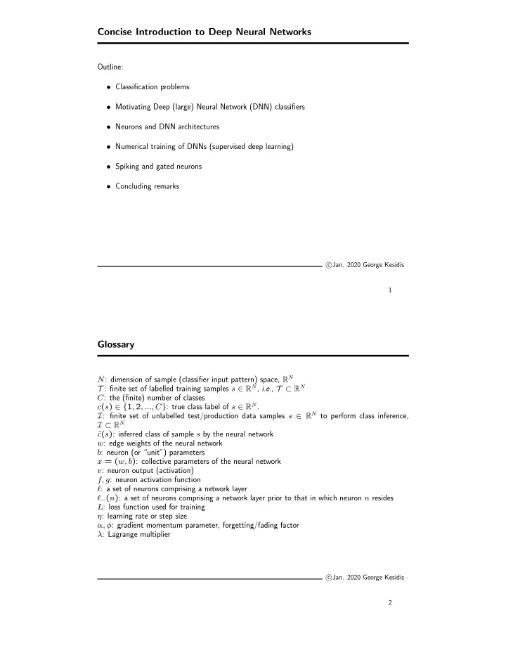
Concise Introduction to Deep Neural Networks Outline: • Classification problems • Motivating Deep (large) Neural Network (DNN) classifiers • Neurons and DNN architectures • Numerical training of DNNs (supervised deep learning) • Spiking and gated neurons • Concluding remarks � Jan. 2020 George Kesidis c 1 Glossary N : dimension of sample (classifier input pattern) space, R N T : finite set of labelled training samples s 2 R N , i.e. , T ⇢ R N C : the (finite) number of classes c ( s ) 2 { 1 , 2 , ..., C } : true class label of s 2 R N . I : finite set of unlabelled test/production data samples s 2 R N to perform class inference, I ⇢ R N ˆ c ( s ) : inferred class of sample s by the neural network w : edge weights of the neural network b : neuron (or “unit”) parameters x = ( w, b ) : collective parameters of the neural network v : neuron output (activation) f, g : neuron activation function ` : a set of neurons comprising a network layer ` � ( n ) : a set of neurons comprising a network layer prior to that in which neuron n resides L : loss function used for training ⌘ : learning rate or step size ↵ , � : gradient momentum parameter, forgetting/fading factor � : Lagrange multiplier � Jan. 2020 George Kesidis c 2

Classification problems • Consider many data samples in a large feature space. • The samples may be, e.g. , images, segments of speech, documents, or the current state of an online game. • Suppose that, based on each sample, one of a finite number of decision must be made. • Plural samples may be associated with the same decision, e.g. , – the type of animal in an image, – the word that is being spoken in a segment of speech, – the sentiment or topic of some text, or – the action that is to be taken by a particular player at a particular state in the game. • Thus, we can define a class of samples as all of those associated with the same decision. � Jan. 2020 George Kesidis c 3 Classifier • A sample s is an input pattern to a classifier. • The output ˆ c ( s ) is the inferred class label (decision) for the sample s . • The classifier parameters x = ( w, b ) need to be learned so that the inferred class decisions are mostly accurate. � Jan. 2020 George Kesidis c 4

Types of data • The samples themselves may have features that are of di ff erent types, e.g. , categorical, discrete numerical, continuous numerical. • There are di ff erent ways to transform data of all types to continuous numerical. • How this is done may significantly a ff ect classification performance. • This is part of an often complex, initial data-preparation phase of DNN training. • In the following, we assume all samples s 2 R N for some feature dimension N . � Jan. 2020 George Kesidis c 5 Training and test datasets for classification • Consider a finite training dataset T ⇢ R N with true class labels c ( s ) for all s 2 T . • T has representative samples of all C classes, c : T ! { 1 , 2 , ..., C } . • Using T , c , the goal is to create a classifier c : R N ! { 1 , 2 , ..., C } that ˆ – accurately classifies on T , i.e. , 8 s 2 T , ˆ c ( s ) = c ( s ) , and – hopefully generalizes well to an unlabelled production/test set I encountered in the field with the same distribution as T , i.e. , hopefully for most s 2 I , ˆ c ( s ) = c ( s ) . • That is, the classifier “infers” the class label of the test samples s 2 I . • To learn decision-making hyperparameters, a held-out subset of the training set, H , with representatives from all classes, may be used to ascertain the accuracy of a classifier ˆ c on H as P s 2 H 1 { ˆ c ( s ) = c ( s ) } ⇥ 100% . |H| � Jan. 2020 George Kesidis c 6

Optimal Bayes error rate • The test/production set I is not available or known during training. • May be some ambiguity when deciding about some samples. • For each sample/input-pattern s , there is a true posterior distribution on the classes p (  | s ) , where p (  | s ) � 0 and P C  =1 p (  | s ) = 1 . • This gives the Bayes error (misclassification) rate, e.g. , Z B := R N (1 � p ( c ( s ) | s )) ( s ) d s, where is the (true) prior density on the input sample-space R N . • A given classifier ˆ c trained on a finite training dataset T (hopefully sampled according to ) may have normalized outputs for each class, ˆ p (  | s ) � 0 , cf. softmax output layers. • The classifier will have error rate Z R N (1 � ˆ p (ˆ c ( s ) | s )) ( s ) d s � B. • See Duda, Hart and Stork. Pattern Classification. 2nd Ed. Wiley, 2001. � Jan. 2020 George Kesidis c 7 Motivating Deep (large) Neural Network (DNN) classifiers • Consider a large training set T ⇢ R N ( |T | � 1 ) in a high-dimensional feature space ( N � 1 ) with a possibly large number of associated classes ( C � 1 ). • In such cases, class decision boundaries may be nonconvex, and each class may consist of multiple disjoint regions (components) in feature space R N . • So a highly parameterized classifier, e.g. , Deep (large) artificial Neural Network (DNN), is warranted. • Note: A ⇢ R N is a convex set i ff 8 x, y 2 A and 8 r 2 [0 , 1] , rx + (1 � r ) y 2 A . � Jan. 2020 George Kesidis c 8

Non-convex classes ⇢ R N single-component classes all convex components, A & B are not convex A is convex class, B & D are not Some alternative classification frameworks: • Gaussian Mixture Models (GMMs) with BIC training objective to select the number of components • Support-Vector Machines (SVMs) 9 Cover’s theorem Theorem: If the classes represented in T ⇢ R N are not linearly separable, then there is a nonlinear mapping µ such that µ ( T ) = { µ ( s ) | s 2 T } are linearly separable. Proof: • Choose an enumeration T = { s (1) , s (2) , ..., s ( K ) } where K = |T | . • Continuously map each sample s to a di ff erent unit vector 2 R K ; • that is, 8 k, µ ( s ( k ) ) = e ( k ) , where e ( k ) = 1 and e ( k ) = 0 8 j 6 = k . k j • For example, use Lagrange interpolating polynomials with 2-norm k · k in R N : K k s � s ( j ) k Y 8 k, µ k ( s ) = k s ( k ) � s ( j ) k , j =1 ,j 6 = k where µ = [ µ 1 , ..., µ K ] T : R N ! R K . c � Jan. 2020 George Kesidis 10

Proof of Cover’s theorem (cont) • Every partition of the samples µ ( T ) = { µ ( s ) | s 2 T } into two di ff erent sets (classes)  1 and  2 is separable by the hyperplane with parameters e ( k ) � e ( k ) (so w 2 R K has entries ± 1 ) . X X w = k 2  1 k 2  2 • Thus, 8 k 2  1 , w T e ( k ) = 1 > 0 , and 8 k 2  2 , w T e ( k ) = � 1 < 0 . • We can build a classifier for C > 2 classes from C such linear, binary classifiers: – Consider partition  1 ,  2 , ...,  C of µ ( T ) . – i th binary classifier separates  i from [ j 6 = i  j , i.e. , “one versus rest”. • Q.E.D. � Jan. 2020 George Kesidis c 11 Cover’s theorem - Remarks • Here, µ ( s ) may be analogous to DNN mapping from input s to an internal layer. • One can roughly conclude from Cover’s theorem that: • If the feature dimension is already much larger than the number of samples ( i.e. , N � K as in, e.g. , some genome datasets), then the data T will likely already be linearly separable. � Jan. 2020 George Kesidis c 12

DNN architectures Outline: • Some types of neurons/units (activation functions) • Some types of layers • Example DNN architectures especially for image classification � Jan. 2020 George Kesidis c 13 Illustrative 4-layer, 2-class neural network (with softmax layer) 14

Some types of neurons • Consider a neuron/unit n in layer ` ( n ) , n 2 ` ( n ) , with input edge-weights w i,n , where neurons i are in layer prior (closer to the input) to that of n , i 2 ` � ( n ) . • The activation of neuron n is 0 1 @ X A , v n = f v i w i,n , b n i 2 ` � ( n ) where b n are additional parameters of the activation itself. • Neurons of the linear type have activation functions of the form f ( z, b n ) = b n, 1 z + b n, 0 , where slope b n, 1 > 0 and b n, 0 is a “bias” parameter. � Jan. 2020 George Kesidis c 15 Sigmoid activation function 1.0 0.8 0.6 0.4 0.2 - 10 - 5 5 10 � Jan. 2020 George Kesidis c 16

Some types of neurons (cont) • Neurons of the sigmoid type have activation functions that include f ( z, b n ) = tanh( zb n, 1 + b n, 0 ) 2 ( � 1 , 1) , or 1 1 + exp( � zb n, 1 � b n, 0 ) 2 (0 , 1) , where b n, 1 > 0 . f ( z, b n ) = • Rectified Linear activations Units (ReLU) type activation functions include f ( z, b n ) = ( b n, 1 z + b n, 0 ) + = max { b n, 1 z + b n, 0 , 0 } . • Note that ReLUs are not continuously di ff erentiable at z = � b n, 0 /b n, 1 . • Also, both linear and ReLU activations are not necessarily bounded, whereas sigmoids are. • “Hard threshold” neural activations involving unit-step functions u ( x ) = 1 { x � 0 } , e.g. , f ( z, b n ) = b n, 0 u ( z � b n, 1 ) � 0 , obviously are not di ff erentiable. • Spiking and gated neuron types are discussed later. � Jan. 2020 George Kesidis c 17 Some types of layers - fully connected • Consider neurons n in layer ` = ` ( n ) . • If it’s possible that w i,n 6 = 0 for all i 2 ` � ( n ) , n 2 ` , then layer ` is said to be fully interconnected . � Jan. 2020 George Kesidis c 18