Concentration for Coulomb gases and Coulomb transport inequalities - PowerPoint PPT Presentation
Concentration for Coulomb gases and Coulomb transport inequalities Myl` ene Ma da U. Lille, Laboratoire Paul Painlev e Joint work with Djalil Chafa and Adrien Hardy U. Paris-Dauphine and U. Lille ICERM, Providence - February
Concentration for Coulomb gases and Coulomb transport inequalities Myl` ene Ma¨ ıda U. Lille, Laboratoire Paul Painlev´ e Joint work with Djalil Chafa¨ ı and Adrien Hardy U. Paris-Dauphine and U. Lille ICERM, Providence - February 2018
Outline of the talk 2
Outline of the talk ◮ Coulomb gases : definition and known results 2
Outline of the talk ◮ Coulomb gases : definition and known results ◮ Concentration inequalities 2
Outline of the talk ◮ Coulomb gases : definition and known results ◮ Concentration inequalities ◮ Outline of the proof and Coulomb transport inequalities 2
Coulomb gases ( d ≥ 2 ) We consider the Poisson equation ∆ g = − c d δ 0 . The fundamental solution is given by � − log | x | for d = 2 , g ( x ) := 1 for d ≥ 3 . | x | d − 2 A gas of N particles interacting according to the Coulomb law would have an energy given by N � � H N ( x 1 , . . . , x N ) := g ( x i − x j ) + N V ( x i ) . i � = j i =1 3
V ,β the Gibbs measure on ( R d ) N associated to this We denote by P N energy : 1 e − β 2 H N ( x 1 ,..., x N ) d x 1 , . . . , d x N d P N V ,β ( x 1 , . . . , x N ) = Z N V ,β 4
V ,β the Gibbs measure on ( R d ) N associated to this We denote by P N energy : 1 e − β 2 H N ( x 1 ,..., x N ) d x 1 , . . . , d x N d P N V ,β ( x 1 , . . . , x N ) = Z N V ,β Example (Ginibre) : let M N be an N by N matrix with iid entries with law N C (0 , 1 N ) , then the eigenvalues have joint law P N | x | 2 , 2 with | x i − x j | 2 e − N � N i =1 | x i | 2 � d P N | x | 2 , 2 ( x 1 , . . . , x N ) ∼ i < j 4
Global asymptotics of the empirical measure 5
Global asymptotics of the empirical measure Our main subject of study is the empirical measure N µ N := 1 � ˆ δ x i . N i =1 5
Global asymptotics of the empirical measure Our main subject of study is the empirical measure N µ N := 1 � ˆ δ x i . N i =1 One can rewrite H N ( x 1 , . . . , x N ) = N 2 E � = V (ˆ µ N ) ��� � � := N 2 g ( x − y )ˆ µ N ( d x )ˆ µ N ( d y ) + V ( x )ˆ µ N ( d x ) . x � = y 5
Global asymptotics of the empirical measure Our main subject of study is the empirical measure N µ N := 1 � ˆ δ x i . N i =1 One can rewrite H N ( x 1 , . . . , x N ) = N 2 E � = V (ˆ µ N ) ��� � � := N 2 g ( x − y )ˆ µ N ( d x )ˆ µ N ( d y ) + V ( x )ˆ µ N ( d x ) . x � = y More generally, one can define, for any µ ∈ P ( R d ) , �� � g ( x − y ) + 1 2 V ( x ) + 1 � E V ( µ ) := 2 V ( y ) µ ( d x ) µ ( d y ) . 5
If V is admissible, there exists a unique minimizer µ V of the functional E V and it is compactly suppported. 6
If V is admissible, there exists a unique minimizer µ V of the functional E V and it is compactly suppported. If V is continuous, one can check that almost surely ˆ µ N converges weakly to µ V . 6
If V is admissible, there exists a unique minimizer µ V of the functional E V and it is compactly suppported. If V is continuous, one can check that almost surely ˆ µ N converges weakly to µ V . A large deviation principle, due to Chafa¨ ı, Gozlan and Zitt is also available : 6
If V is admissible, there exists a unique minimizer µ V of the functional E V and it is compactly suppported. If V is continuous, one can check that almost surely ˆ µ N converges weakly to µ V . A large deviation principle, due to Chafa¨ ı, Gozlan and Zitt is also available : for d a distance that metrizes the weak topology (for example Fortet-Mourier) one has in particular 1 N →∞ − β N 2 log P N V ,β ( d (ˆ µ N , µ V ) ≥ r ) − − − − → d ( µ,µ V ) ≥ r ( E V ( µ ) − E V ( µ V )) . inf 2 6
If V is admissible, there exists a unique minimizer µ V of the functional E V and it is compactly suppported. If V is continuous, one can check that almost surely ˆ µ N converges weakly to µ V . A large deviation principle, due to Chafa¨ ı, Gozlan and Zitt is also available : for d a distance that metrizes the weak topology (for example Fortet-Mourier) one has in particular 1 N →∞ − β N 2 log P N V ,β ( d (ˆ µ N , µ V ) ≥ r ) − − − − → d ( µ,µ V ) ≥ r ( E V ( µ ) − E V ( µ V )) . inf 2 What about concentration ? 6
If V is admissible, there exists a unique minimizer µ V of the functional E V and it is compactly suppported. If V is continuous, one can check that almost surely ˆ µ N converges weakly to µ V . A large deviation principle, due to Chafa¨ ı, Gozlan and Zitt is also available : for d a distance that metrizes the weak topology (for example Fortet-Mourier) one has in particular 1 N →∞ − β N 2 log P N V ,β ( d (ˆ µ N , µ V ) ≥ r ) − − − − → d ( µ,µ V ) ≥ r ( E V ( µ ) − E V ( µ V )) . inf 2 What about concentration ? Local behavior extensively using several variations of the concept of renormalized energy (see in particular Simona’s talk this morning). 6
Concentration estimates 7
Concentration estimates We will consider both the bounded Lipschitz distance d BL and the Wassertein W 1 distance, where we recall that � � d BL ( µ, ν ) = sup f d ( µ − ν ); W 1 ( µ, ν ) = sup f d ( µ − ν ) � f � ∞ ≤ 1 � f � Lip ≤ 1 � f � Lip ≤ 1 7
Concentration estimates We will consider both the bounded Lipschitz distance d BL and the Wassertein W 1 distance, where we recall that � � d BL ( µ, ν ) = sup f d ( µ − ν ); W 1 ( µ, ν ) = sup f d ( µ − ν ) � f � ∞ ≤ 1 � f � Lip ≤ 1 � f � Lip ≤ 1 Theorem If V is C 2 and V and ∆ V satisfy some growth conditions, 7
Concentration estimates We will consider both the bounded Lipschitz distance d BL and the Wassertein W 1 distance, where we recall that � � d BL ( µ, ν ) = sup f d ( µ − ν ); W 1 ( µ, ν ) = sup f d ( µ − ν ) � f � ∞ ≤ 1 � f � Lip ≤ 1 � f � Lip ≤ 1 Theorem If V is C 2 and V and ∆ V satisfy some growth conditions,then there exist a > 0 , b ∈ R , c ( β ) such that for all N ≥ 2 and for all r > 0 , 4 N log N + b β N 2 − 2 µ N , µ V ) ≥ r ) ≤ e − a β N 2 r 2 + 1 d =2 β d + c ( β ) N P N V ,β ( d (ˆ 7
More insight about the growth conditions : 8
More insight about the growth conditions : ◮ ∆ V has to grow not faster then V 8
More insight about the growth conditions : ◮ ∆ V has to grow not faster then V ◮ as soon as the model is well defined, the concentration estimate holds for d BL 8
More insight about the growth conditions : ◮ ∆ V has to grow not faster then V ◮ as soon as the model is well defined, the concentration estimate holds for d BL ◮ if moreover V ( x ) � c | x | κ , for some κ > 0 , we can say more about c ( β ) near 0 and near ∞ 8
More insight about the growth conditions : ◮ ∆ V has to grow not faster then V ◮ as soon as the model is well defined, the concentration estimate holds for d BL ◮ if moreover V ( x ) � c | x | κ , for some κ > 0 , we can say more about c ( β ) near 0 and near ∞ ◮ if moreover V ( x ) � c | x | 2 , the concentration estimate holds for W 1 8
More insight about the growth conditions : ◮ ∆ V has to grow not faster then V ◮ as soon as the model is well defined, the concentration estimate holds for d BL ◮ if moreover V ( x ) � c | x | κ , for some κ > 0 , we can say more about c ( β ) near 0 and near ∞ ◮ if moreover V ( x ) � c | x | 2 , the concentration estimate holds for W 1 ◮ the latter allows to get the almost sure convergence of µ N , µ V ) to zero down to β ≃ log N W 1 (ˆ N 8
More insight about the growth conditions : ◮ ∆ V has to grow not faster then V ◮ as soon as the model is well defined, the concentration estimate holds for d BL ◮ if moreover V ( x ) � c | x | κ , for some κ > 0 , we can say more about c ( β ) near 0 and near ∞ ◮ if moreover V ( x ) � c | x | 2 , the concentration estimate holds for W 1 ◮ the latter allows to get the almost sure convergence of µ N , µ V ) to zero down to β ≃ log N W 1 (ˆ N ◮ if the potential is subquadratic, a , b and c ( β ) can be made more explicit. 8
A few more comments : 9
A few more comments : ◮ Possible rewriting : there exist r 0 , C > 0 , such that for all N ≥ 2 , if � � log N if d = 2 r 0 r ≥ N r 0 N − 1 / d if d ≥ 3 , µ N , µ V ) ≥ r ) ≤ e − CN 2 r 2 . P N V ,β ( d (ˆ 9
A few more comments : ◮ Possible rewriting : there exist r 0 , C > 0 , such that for all N ≥ 2 , if � � log N if d = 2 r 0 r ≥ N r 0 N − 1 / d if d ≥ 3 , µ N , µ V ) ≥ r ) ≤ e − CN 2 r 2 . P N V ,β ( d (ˆ ◮ thanks to the large deviation results of CGZ, we know that we are in the right scale 9
A few more comments : ◮ Possible rewriting : there exist r 0 , C > 0 , such that for all N ≥ 2 , if � � log N if d = 2 r 0 r ≥ N r 0 N − 1 / d if d ≥ 3 , µ N , µ V ) ≥ r ) ≤ e − CN 2 r 2 . P N V ,β ( d (ˆ ◮ thanks to the large deviation results of CGZ, we know that we are in the right scale ◮ for Ginibre, the constants can be computed explicitely ; improves on previous results based on determinantal structure (can we use the Gaussian nature of the entries ?) 9
Recommend
More recommend
Explore More Topics
Stay informed with curated content and fresh updates.
