Computing Second Order Derivatives with ADiMat Facilitating Optimal - PowerPoint PPT Presentation

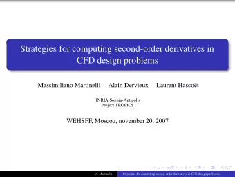
Introduction Second Order Derivatives with ADiMat Performance Results Summary Computing Second Order Derivatives with ADiMat Facilitating Optimal Experimental Design by Automatic Differentiation Johannes Willkomm Institute for Scientific Computing Technische Universität Darmstadt May 14, 2013 / Colloquium of the Interdisciplinary Center for Scientific Computing (IWR) of Heidelberg University

Introduction Second Order Derivatives with ADiMat Performance Results Summary Outline Introduction 1 Second Order Derivatives ADiMat Second Order Derivatives with ADiMat 2 Full Second Order Derivatives: Hessians Nested Application of ADiMat Performance Results 3

Introduction Second Order Derivatives with ADiMat Performance Results Summary Second Order Derivatives Second Order Derivatives Second order derivatives are often required in software for Optimal Experimental Design (OED), for example in VPLAN [Körkel, 2002]. We consider functions of the form z = F ( x , p , q ) : ( R n x × R n p × R n q ) → R m Costs: time T F and memory M F Needed derivatives: d 2 F d 2 F d 2 F d x 2 , d x d q , and d p d q Abbreviations: X = [ x , p , q ] , n = n x + n p + n q Using Automatic Differentiation (AD) for 2 nd order derivatives is attractive for performance reasons Precise derivatives help in optimization AD is often more efficient than numerical methods AD is more broadly applicable (in the mathematical sense)

Introduction Second Order Derivatives with ADiMat Performance Results Summary Second Order Derivatives Example Function function z = F( x , p , q ) t1 = 1; for i =1: length ( x ) t1 = t1 . ∗ sin ( x ( i ) ) ; end t2 = 1; for i =1: length ( p ) t2 = t2 . ∗ sin ( x ( i ) . ∗ q ( i ) ) ; end t3 = 1; for i =1: length ( q ) t3 = t3 . ∗ cos ( p ( i ) . ∗ q ( i ) ) ; end z = [ t1 , t2 , t3 ] ;

Introduction Second Order Derivatives with ADiMat Performance Results Summary Second Order Derivatives 2 nd Order Derivatives of Example Function d 2 F d 2 F d 2 F d x 2 d x d q d p d q 0 0 0 5 5 5 10 10 10 15 15 15 20 20 20 25 25 25 30 30 30 0 10 20 30 0 10 20 30 0 10 20 30 (a) d 2 z 1 (b) d 2 z 2 (c) d 2 z 3 d X 2 d X 2 d X 2 Figure: spy plots of the Hessians of the m = 3 output components of F for n x = n p = n q = 10 .

Introduction Second Order Derivatives with ADiMat Performance Results Summary ADiMat ADiMat A utomatic Di fferentiation for Mat lab ( ADiMat ) is an AD tool for MATLAB (http://www.adimat.de) Uses source transformation, but combines it with operator overloading [Bischof & Bücker et al., 2002] Supports both forward mode (FM) and reverse mode (RM) Capitalizes on the high-level mathematical functions and operators in MATLAB, like ∗ , \ , eig , svd , expm , cross , interp1 , roots , . . . ADiMat features Comfortable user interface [Willkomm & Bischof & Bücker, 2012] Higher order derivatives (univariate and mixed)

Introduction Second Order Derivatives with ADiMat Performance Results Summary ADiMat ADiMat Internals ADiMat transforms function F to a new function function z = F(a , b ) z = a ∗ b ; admDiffFor admDiffRev function [ g_z , z ]= g_F ( g_a , a , g_b , b ) function [ a_a a_b nr_z ] = a_F (a , b , a_z ) g_z= g_a ∗ b+ a ∗ g_b ; z = a ∗ b ; z= a ∗ b ; nr_z = z ; [ a_a a_b ] = a_zeros (a , b ) ; a_a = a_a + a_z ∗ b . ’ ; a_b = a_b + a . ’ ∗ a_z ; end Evaluation of derivatives of F at certain arguments a, b by running the generated functions Derivative inputs have to be properly initialized (seeding)

Introduction Second Order Derivatives with ADiMat Performance Results Summary ADiMat Scalar and Vector Mode Derivative variables have the same shape as the originals This only allows for a single directional g_a b * derivative in g_x : scalar mode For vector mode use derivative class objects, with overloaded operators, as containers for n dd > 1 directional derivatives Overloaded operator dispatch happens at run time, since MATLAB is weakly g_a * b typed Performance is quite bad

Introduction Second Order Derivatives with ADiMat Performance Results Summary ADiMat Alternative: Vectorized Code Alternative: “vectorize” the code explicitly Replace objects by opaque data type Replace overloaded operators by function calls function [ d_z z ] = d_F ( d_a , a , d_b , b ) admDiffVFor function z = F(a , b ) d_z = opdiff_mult ( d_a , a , d_b , b ) ; z = a ∗ b ; z = a ∗ b ; end Resolution of function calls now at compile time Often very good performance, especially with “scalar” or “F77-style” codes, for small to medium n dd .

Introduction Second Order Derivatives with ADiMat Performance Results Summary Driver for Hessians Full 2 nd Order Derivatives: Hessians Main driver for second order derivatives is admHessian Computes the full Hessian matrix H or (multiple) products H · v thereof We can pick out our desired derivatives from H , or compute only the suitable linear combinations H · v Returns the Hessians of all function results H k , 1 ≤ k ≤ m Two evaluation strategies: Forward over reverse mode (default) Linear combination of second order univariate Taylor coefficients

Introduction Second Order Derivatives with ADiMat Performance Results Summary Driver for Hessians Forward over Reverse Mode Differentiate function F in RM Run RM evaluation with a typical first order FM OO class Obtain first order derivatives of function result by the FM and the derivatives of those w.r.t. all inputs by the RM Costs: Time O ( m ) · T F for one H · v product Time O ( n · m ) · T F for full H Space O ( T F ) for the stack required by the RM adopts = admOptions ( ’ i ’ , [1 2 3 ] ) ; adopts . functionResults = { z } ; H = admHessian (@F, 1 , x , p , q , adopts ) ; Caveat: FM OO class supports very few builtins as of yet

Introduction Second Order Derivatives with ADiMat Performance Results Summary Driver for Hessians Forward over Reverse Mode We don’t need the full Hessian H , in particular not d 2 F d q 2 Mask out the columns corresp. to q with a seed matrix   I n x 0 n p  ∈ R n × ( n x + n p ) S = 0 n p I n p  0 n q 0 n q With the example function F we could even use compression (adding together the x – and p –columns) Costs: Time O (( n x + n p ) · m ) · T F for the desired sub blocks of H S = [ eye ( numel ( x ) ) zeros ( numel ( x ) ) zeros ( numel ( p ) ) eye ( numel ( p ) ) zeros ( numel ( q ) ) zeros ( numel ( q ) ) ] ; H = admHessian (@F, S, x , p , q , adopts ) ;

Introduction Second Order Derivatives with ADiMat Performance Results Summary Driver for Hessians 2 nd Order Taylor Coefficients Propagate 2 nd order univariate Taylor coefficients in FM Compute the off-diagonal Hessian entries as � � H i , j = 1 D 2 e i + e j F ( X ) − D 2 e i F ( X ) − D 2 e j F ( X ) , i � = j 2 [Griewank & Walther, 2008] For full H need n + n · ( n + 1 ) derivative directions 2 Costs: Time O ( n 2 ) · T F for full H Space O ( n 2 ) · M F adopts . hessianStrategy = ’ t 2 f o r ’ ; % A l t e r n a t i v e s : use FD, vectorized Taylor mode % adopts . admDiffFunction = @admDiffFD ; % adopts . admDiffFunction = @admTaylorVFor ; H = admHessian (@F, 1 , x , p , q , adopts ) ;

Introduction Second Order Derivatives with ADiMat Performance Results Summary Nested Application of ADiMat Mixed 2 nd Order Directional Derivatives Generate three functions by twice applying the FM Diff. F in FM w.r.t. x , then dx_F w.r.t. both x and g_x Also differentiate dx_F w.r.t. q Differentiate F in FM w.r.t. p , then dp_F w.r.t. q alias ac= ’ adimat − c l i e n t − F ’ ac − i x − d1 − odx_F .m F .m ac − ig_x , x − d1 − sgradprefix=h_ − odx_dx_F .m dx_F .m ac − iq − d1 − sgradprefix=h_ − odq_dx_F .m dx_F .m ac − ip − d1 − odp_F .m F .m ac − iq − d1 − sgradprefix=h_ − odq_dp_F .m dp_F .m Costs: Time O ( 1 ) · T F and space O ( 1 ) · M F for one entry H i , j Time O ( n 2 x / 2 + n x n q + n p n q ) · T F for the desired sub blocks Caveat: ADiMat may not be able to reprocess its code

Introduction Second Order Derivatives with ADiMat Performance Results Summary Nested Application of ADiMat Mixed 2 nd Order Directional Derivatives h_g_x = zeros ( size ( x ) ) ; h_x = h_g_x ; g_x = h_x ; for i =1: numel ( x ) , for j =1: i h_x ( i ) = 1; g_x ( j ) = 1; h_g_f = dx_dx_F ( h_g_x , g_x , h_x , x , p , q ) ; dF_dxdx ( : , i , j ) = h_g_f ( : ) ; dF_dxdx ( : , j , i ) = h_g_f ( : ) ; h_x ( i ) = 0; g_x ( j ) = 0; end end h_q = zeros ( size ( q ) ) ; g_x = zeros ( size ( x ) ) ; for i =1: numel ( x ) , for j =1: numel ( q ) g_x ( i ) = 1; h_q ( j ) = 1; h_g_f = dq_dx_F ( g_x , x , p , h_q , q ) ; dF_dqdx ( : , i , j ) = h_g_f ( : ) ; g_x ( i ) = 0; h_q ( j ) = 0; end end % likewise f o r dF_dqdp

Introduction Second Order Derivatives with ADiMat Performance Results Summary Nested Application of ADiMat Complex Variable Method over FM First order FM to compute Jacobian Apply complex variable (CV) method on top of that Only applicable if F is real analytic Very precise and efficient approximation to derivatives adopts2 = admOptions ( ’ i ’ , [1 2 3] + 2 , ’d ’ , 1 ) ; adopts2 . nargout = 1; H = admDiffComplex (@ admDiffVFor , S, . . . @F, 1 , x , p , q , adopts , adopts2 ) ; H = reshape (H, [ numel ( z ) size (S ) ] ) ; Costs: Time O ( n ) · T F for one H · v product Time O ( n · ( n x + n p )) · T F for the desired sub blocks of H Space O ( n ) · M F