Computer Graphics CS 543 Lecture 4 (Part 3) Introduction to - PowerPoint PPT Presentation
Computer Graphics CS 543 Lecture 4 (Part 3) Introduction to Transformations (Part 2) Prof Emmanuel Agu Computer Science Dept. Worcester Polytechnic Institute (WPI) Introduction to Transformations Transformation changes an objects: Position
Computer Graphics CS 543 – Lecture 4 (Part 3) Introduction to Transformations (Part 2) Prof Emmanuel Agu Computer Science Dept. Worcester Polytechnic Institute (WPI)
Introduction to Transformations Transformation changes an objects: Position (translation) Size (scaling) Orientation (rotation) Shapes (shear) Introduce first in 2D or (x,y) , build intuition Later, talk about 3D Transform object by applying sequence of matrix multiplications to object vertices
Transformations in OpenGL Pre 3.0 OpenGL had a set of transformation functions (now deprecated) glTranslate( ) glRotate( ) glScale( )
Transformations in OpenGL OpenGL would previously receive transform commands, maintain concatenations of transform matrices as modelview matrix No longer Programmer *may* now choose to maintain modelview or NOT!
Transformations in OpenGL Three choices Application code GLSL functions vec.h and mat.h
Why Matrices? All transformations can be performed using matrix/vector multiplication Allows pre ‐ multiplication of all matrices Note: point (x,y) needs to be represented as (x,y,1), also called Homogeneous coordinates
Homogenous Coordinates Homogeneous coordinates representation of point P = (Px,Py,Pz) => (Px,Py,Pz,1) We could introduce arbitrary scaling factor, w, so that P = (wPx, wPy, wPz, w) ( Note: w is non ‐ zero) For example, the point P = (2,4,6) can be expressed as (2,4,6,1) or (4,8,12,2) where w=2 or (6,12,18,3) where w = 3, or…. To convert from homogeneous back to ordinary coordinates, first divide all four terms by w and discard 4 th term
Homogeneous Coordinates and Computer Graphics Homogeneous coordinates are key in graphics Transformations (rotation, translation, scaling) can be implemented with matrix multiplications using 4 x 4 matrices Hardware pipeline works with 4 dimensional representations
The World Frames In OpenGL, objects/scene initially defined in world frame Transformations (translate, scale, rotate) applied to objects in world frame World frame (Origin at 0,0,0)
Camera Frame After we define a camera (eye) position We then represent objects in camera frame (origin at eye position) objects moved from world frame to camera frame using model ‐ view matrix World frame (Origin at 0,0,0) Camera frame (Origin at camera)
General Transformations A transformation maps points to other points and/or vectors to other vectors v=T(u) Q=T(P)
Affine Transformations Rigid body transformations: rotation, translation, scaling, shear Line preserving: i mportant in graphics since we can Transform endpoints of line segments 1. Draw line segment between the transformed endpoints 2.
Pipeline Implementation T (from application program) frame u T(u) buffer transformation rasterizer v T(v) T(v) T(v) v T(u) u T(u) vertices pixels vertices
Point Representation We use a column matrix (2x1 matrix) to represent a 2D point x y General form of transformation of a point (x,y) to (x’,y’) can be written as: x ' ax by c x ' a b c x y ' d e f y or 1 0 0 1 1 y ' dx ey f
Translation To reposition a point along a straight line Given point (x,y) and translation distance (t x , t y ) The new point: (x’,y’) (x’,y’) x’=x + t x y’=y + t y (x,y) or x ' x t y x P where P ' P ' P T T ' y t y
3x3 2D Translation Matrix t x ' x x t y ' y y use 3x1 vector x x ' 1 0 t x y y ' 0 1 t * y 1 1 0 0 1 Note: it becomes a matrix-vector multiplication
2D Translation of Objects How to translate an object with multiple vertices? t y = 3 Translate individual vertices t x = 3 0 . 5 x ' 1 0 3 0 . 5 y ' 0 1 3 * 1 1 0 0 1
3D Translation Move each vertex by same distance d = (d x , d y , d z ) object translation: every point displaced by same vector
Transforms in 3D 2D: 3x3 matrix multiplication 3D: 4x4 matrix multiplication: homogenous coordinates Again: transform object = transform each vertice General form: m m m m Q P 11 12 13 14 x x Xform of P m m m m Q P 21 22 23 24 y y M M m m m m Q P 31 32 33 34 z z 0 0 0 1 1 1
3D Translation Matrix Now, 3D : x t x ' x y t y ' y z t z ' z translate(tx,ty,tz) x x ' 1 0 0 t x y y ' 0 1 0 t y * z z ' 0 0 1 t z 1 1 0 0 0 1 Where: x’= x.1 + y.0 + z.0 + tx.1 = x + tx , … etc
2D Scaling Scale: Alter object size by scaling factor (s x , s y ). i.e ' 0 x Sx x x’ = x . Sx y’ = y . Sy y ' 0 Sy y (4,4) Sx = 2, Sy = 2 (2,2) (2,2) (1,1)
2D Scaling Matrix x ' Sx 0 x y ' 0 Sy y x ' Sx 0 0 x y ' 0 Sy 0 y 1 0 0 1 1
Scaling Expand or contract along each axis (fixed point of origin) x’=s x x y’=s y x z’=s z x p ’= Sp s 0 0 0 x 0 s 0 0 y S = S (s x , s y , s z ) = 0 0 s 0 z 0 0 0 1
4x4 3D Scaling Matrix x ' Sx 0 0 x y ' 0 Sy 0 y Scale(Sx,Sy,Sz) 1 0 0 1 1 •Example: •If Sx = Sy = Sz = 0.5 •Can scale: • big cube (sides = 1) to x ' S 0 0 0 x small cube ( sides = 0.5) x •2D: square, 3D cube y ' 0 S 0 0 y y z ' 0 0 S 0 z z 1 0 0 0 1 1
Shearing y*h x (x,y) (x + y*h, y) Y coordinates are unaffected, but x cordinates are translated linearly with y That is: y’ = y x 1 h 0 x x’ = x + y * h y 0 1 0 y 1 0 0 1 1 h is fraction of y to be added to x
3D Shear
Reflection corresponds to negative scale factors s x = -1 s y = 1 original s x = -1 s y = -1 s x = 1 s y = -1
References Angel and Shreiner Hill and Kelley
Recommend
More recommend
Explore More Topics
Stay informed with curated content and fresh updates.

