Computational Learning Theory Based on Machine Learning, T. - PowerPoint PPT Presentation

0. Computational Learning Theory Based on “Machine Learning”, T. Mitchell, McGRAW Hill, 1997, ch. 7 Acknowledgement: The present slides are an adaptation of slides drawn by T. Mitchell

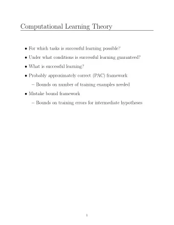
1. Main Questions in Computational Learning Theory • Can one characterize the number of training examples nec- essary/sufficient for successful learning? ◦ Is it possible to identify classes of concepts that are inher- ently difficult/easy to learn, independent of the learning algorithm?

2. We seek answers in terms of • sample complexity: number of needed training examples ◦ computational complexity: time needed for a learner to converge (with high probability) to a successful hypothesis ◦ the manner in which training examples should be pre- sented to the learner • mistake bound: number of mistakes made by the learner before eventually succeeding

3. Remarks 1. Since no general answers to the above questions are yet known, we will give some key results for particular settings. 2. We will restrict the presentation to inductive learning, in a universe of instances X , in which we learn a target function c from a number of examples D , searching a candidate h in a given hypothesis space H .

4. Plan 1. The Probably Approximately Correct learning model 1.1 PAC-Learnable classes of concepts 1.2 Sample complexity Sample complexity for finite hypothesis spaces Sample complexity for infinite hypothesis spaces 1.3 The Vapnik-Chervonenkis (VC) dimension 2. The Mistake Bound model of learning • The Halving learning algorithm • The Weighted-Majority learning algorithm ◦ The optimal Mistake Bounds

5. 1. The PAC learning model Note: For simplicity, here we restrict the presentation to learning boolean functions, using noisy free training data. Extensions: ◦ considering real-valued functions: [ Natarajan, 1991 ] ; ◦ considering noisy data: [ Kearns & Vazirani, 1994 ] .

6. The True Error of a Hypothesis: error D ( h ) Instance space X x ∈D [ c ( x ) � = h ( x )] Pr - - c h the probability that h will + misclassify a single in- + stance drawn at random according to the distribu- - Where c tion D . and h disagree Note: error D ( h ) is not directly observable to the learner; it can only see the training error of each hypothesis (i.e., how often h ( x ) � = c ( x ) over training instances). Question: Can we bound error D ( h ) given the training error of h ?

7. Important Note Ch. 5 ( Evaluating Hypotheses ) explores the relationship be- tween true error and sample error , given a sample set S and a hypothesis h , with S independent of h . When S is the set of training examples from which h has been learned (i.e., D ), obviously h is not independent of S . Here we deal with this case.

8. The Need for Approximating the True Error of a Hypothesis Suppose that we would like to get a hypothesis h with true error 0: 1. the learner should choose among hypotheses having the training error 0, but since there may be several such candidates, it cannot be sure which one to choose 2. as training examples are drawn randomly, there is a non-0 proba- bility that they will mislead the learner Consequence: demands on the learner should be weakened 1. let error D ( h ) < ǫ with ǫ arbitrarily small 2. not every sequence of training examples should succeed, but only with probability 1 − δ , with δ arbitrarily small

9. 1.1 PAC Learnable Classes of Concepts: Definition Consider a class C of possible target concepts defined over a set of instances X of length n , and a learner L using the hypothesis space H . C is PAC-learnable by L using H if for all c ∈ C , distributions D over X , ǫ such that 0 < ǫ < 1 / 2 , and δ such that 0 < δ < 1 / 2 , the learner L will with probability at least (1 − δ ) output a hypothesis h ∈ H such that error D ( h ) ≤ ǫ , in time that is polynomial in 1 /ǫ , 1 /δ , n and size ( c ) , where size ( c ) is the encoding length of c , assuming some representation for C .

10. PAC Learnability: Remarks (I) ◦ If C is PAC-learnable, and each training example is processed in polynomial time, then each c ∈ C can be learned from a polynomial number of training examples. • Usually, to show that a class C is PAC-learnable, we show that each c ∈ C can be learned from a polynomial number of examples, and the processing time for each example is polynomially bounded.

11. PAC Learnability: Remarks (II) ◦ Unfortunately , we cannot ensure that H contains (for any ǫ, δ ) an h as in the difinition of PAC-learnability unless C is known in advance, or H ≡ 2 X . • However , PAC-learnability provides useful insights on the relative complexity of different ML problems, and the rate at which generalization accuracy improves with additional training examples.

12. 1.2 Sample Complexity In practical applications of machine learning, evaluating the sample com- plexity (i.e. the number of needed training examples) is of greatest interest because in most practical settings limited success is due to limited available training data. We will present results that relate (for different setups) • the size of the instance space ( m ) to • the accuracy to which the target concept is approximated ( ǫ ) • the probability of successfully learning such an hypothesis (1 − δ ) • the size of the hypothesis space ( | H | )

13. 1.2.1 Sample Complexity for Finite Hypothesis Spaces First, we will present a general bound on the sample com- plexity for consistent learners, i.e. which perfectly fit the training data. Recall the version space notion: V S H,D = { h ∈ H |∀� x, c ( x ) � ∈ D, h ( x ) = c ( x ) } Later, we will consider agnostic learning, which accepts the fact that a zero training error hypothesis cannot always be found.

14. Exhaustion of the Version Space Definition: V S H,D is ǫ -exhausted with respect to the target concept c and the training set D if error D ( h ) < ǫ , ∀ h ∈ V S H,D . Hypothesis space H error =.3 error =.1 r =.4 =.2 r error =.2 =0 r VSH,D error =.2 error =.3 =.3 r error =.1 =.1 r =0 r r = training error, error = true error

15. How many examples will ǫ -exhaust the VS? Theorem: [ Haussler, 1988 ] If the hypothesis space H is finite, and D is a sequence of m ≥ 1 independent random examples of some target concept c ∈ H , then for any 0 ≤ ǫ ≤ 1 , the probability that V S H,D is not ǫ -exhausted (with respect to c ) is less than | H | e − ǫm Proof: Let h be a hypothesis of true error ≥ ǫ . The proba- bility that h is consistent with the m independently drawn training examples is < (1 − ǫ ) m . The probability that there are such hypothesis h in H is < | H | (1 − ǫ ) m . As 1 − ǫ ≤ e − ǫ for ∀ ǫ ∈ [0 , 1] , it follows that | H | (1 − ǫ ) m ≤ | H | e − ǫm .

16. Consequence: The above theorem bounds the probability that any consistent learner will output a hypothesis h with error D ( h ) ≥ ǫ . If we want this probability to be below δ | H | e − ǫm ≤ δ then m ≥ 1 ǫ (ln | H | + ln(1 /δ )) This is the number of training examples sufficient to en- sure that any consistent hypothesis will be probably (with probability 1 − δ ) approximately (within error ǫ ) correct.

17. Example 1: EnjoySport If H is as given in EnjoySport (see Chapter 2) then | H | = 973 , and m ≥ 1 ǫ (ln 973 + ln(1 /δ )) If want to assure that with probability 95%, V S contains only hypotheses with error D ( h ) ≤ 0 . 1 , then it is sufficient to have m examples, where m ≥ 1 0 . 1(ln 973+ln(1 /. 05)) = 10(ln 973+ln 20) = 10(6 . 88+3 . 00) = 98 . 8

18. Example 2: Learning conjunctions of boolean literals Let H be the hypothesis space defined by conjunctions of lit- erals based on n boolean attributes possibly with negation. Question: How many examples are sufficient to assure with probability of at least (1 − δ ) that every h in V S H,D satisfies error D ( h ) ≤ ǫ ? Answer: | H | = 3 n , and using our theorem it follows that m ≥ 1 ǫ (ln 3 n + ln(1 /δ )) or m ≥ 1 ǫ ( n ln 3 + ln(1 /δ )) In particular, as Find-S spends O ( n ) time to process one (pos- itive) example, it follows that it PAC-learns the class of conjunctions of n literals with negation.

19. Example 3: PAC-Learnability of k -term DNF expressions k -term DNF expressions: T 1 ∨ T 2 ∨ . . . ∨ T k where T i is a con- junction of n attributes possibly using negation. If H = C then | H | = 3 nk , therefore m ≥ 1 ǫ ( nk ln 3 + ln 1 δ ) , which is polynomial, but... it can be shown (through equivalence with other problems) that it cannot be learned in polynomial time (unless RP � = NP ) therefore k -term DNF expressions are not PAC-learnable.

20. Example 4: PAC-Learnability of k -CNF expressions k -CNF expressions are of form T 1 ∧ T 2 ∧ . . . ∧ T j where T i is a disjunction of up to k boolean attributes. Remark: k -term DNF expressions ⊂ k -CNF expressions. Surprisingly, k -CNF expressions are PAC-learnable by a poly- nomial time complexity algorithm (see [ Vazirani, 1994 ] ). Consequence: k -term DNF expressions are PAC-learnable by an efficient algorithm using H = k -CNF(!).

21. Example 5: PAC-Learnability of Unbiased Learners In such a case, H = C = P ( X ) . If the instances in X are described by n boolean features, then | X | = 2 n and | H | = | C | = 2 | X | = 2 2 n , ǫ (2 n ln 2 + ln 1 therefore m ≥ 1 δ ) Remark: Although the above bound is not a tight one, it can be shown that the sample complexity for learning the unbiased concept class is indeed exponential in n .