La th eorie PAC-Bayes en apprentissage supervis e Pr esentation - PowerPoint PPT Presentation

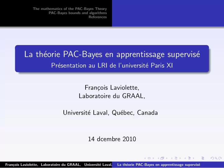
The mathematics of the PAC-Bayes Theory PAC-Bayes bounds and algorithms References La th´ eorie PAC-Bayes en apprentissage supervis´ e Pr´ esentation au LRI de l’universit´ e Paris XI Fran¸ cois Laviolette, Laboratoire du GRAAL, Universit´ e Laval, Qu´ ebec, Canada 14 dcembre 2010 Fran¸ cois Laviolette, Laboratoire du GRAAL, Universit´ e Laval, Qu´ La th´ ebec, Canada eorie PAC-Bayes en apprentissage supervis´ e

The mathematics of the PAC-Bayes Theory PAC-Bayes bounds and algorithms References Summary Aujourd’hui, j’ai l’intention de vous pr´ esenter les math´ ematiques qui sous tendent la th´ eorie PAC-Bayes vous pr´ esenter des algorithmes qui consistent en la minimisation d’une borne PAC-Bayes et comparer ces derniers avec des algorithmes existants. Fran¸ cois Laviolette, Laboratoire du GRAAL, Universit´ e Laval, Qu´ La th´ ebec, Canada eorie PAC-Bayes en apprentissage supervis´ e

The mathematics of the PAC-Bayes Theory PAC-Bayes bounds and algorithms Derivation of classical PAC-Bayes bound References Definitions Each example ( x , y ) ∈ X × {− 1 , +1 } , is drawn acc. to D . The (true) risk R ( h ) and training error R S ( h ) are defined as: m = 1 � def def R ( h ) = ( x , y ) ∼ D I ( h ( x ) � = y ) E ; R S ( h ) I ( h ( x i ) � = y i ) . m i =1 The learner’s goal is to choose a posterior distribution Q on a space H of classifiers such that the risk of the Q -weighted majority vote B Q is as small as possible. � � def B Q ( x ) = sgn h ∼ Q h ( x ) E B Q is also called the Bayes classifier . Fran¸ cois Laviolette, Laboratoire du GRAAL, Universit´ e Laval, Qu´ La th´ ebec, Canada eorie PAC-Bayes en apprentissage supervis´ e

The mathematics of the PAC-Bayes Theory PAC-Bayes bounds and algorithms Derivation of classical PAC-Bayes bound References The Gibbs clasifier PAC-Bayes approach does not directly bounds the risk of B Q It bounds the risk of the Gibbs classifier G Q : to predict the label of x , G Q draws h from H and predicts h ( x ) The risk and the training error of G Q are thus defined as: R ( G Q ) = h ∼ Q R ( h ) ; R S ( G Q ) = h ∼ Q R S ( h ) . E E Fran¸ cois Laviolette, Laboratoire du GRAAL, Universit´ e Laval, Qu´ La th´ ebec, Canada eorie PAC-Bayes en apprentissage supervis´ e

The mathematics of the PAC-Bayes Theory PAC-Bayes bounds and algorithms Derivation of classical PAC-Bayes bound References G Q , B Q , and KL ( Q � P ) If B Q misclassifies x , then at least half of the classifiers (under measure Q ) err on x . Hence: R ( B Q ) ≤ 2 R ( G Q ) Thus, an upper bound on R ( G Q ) gives rise to an upper bound on R ( B Q ) PAC-Bayes makes use of a prior distribution P on H . The risk bound depends on the Kullback-Leibler divergence : h ∼ Q ln Q ( h ) def KL ( Q � P ) = E P ( h ) . Fran¸ cois Laviolette, Laboratoire du GRAAL, Universit´ e Laval, Qu´ La th´ ebec, Canada eorie PAC-Bayes en apprentissage supervis´ e

The mathematics of the PAC-Bayes Theory PAC-Bayes bounds and algorithms Derivation of classical PAC-Bayes bound References A PAC-Bayes bound to rule them all ! , J.R.R. Tolkien, roughly or John Langford, less roughly. Theorem 1 Germain et al. 2009 For any distribution D on X × Y , for any set H of classifiers, for any prior distribution P of support H , for any δ ∈ (0 , 1], and for any convex function D : [0 , 1] × [0 , 1] → R , we have � ∀ Q on H : D ( R S ( G Q ) , R ( G Q )) ≤ Pr S ∼ D m 1 � � 1 ��� h ∼ P e m D ( R S ( h ) , R ( h )) KL ( Q � P ) + ln δ E E m S ∼ D ≥ 1 − δ . Fran¸ cois Laviolette, Laboratoire du GRAAL, Universit´ e Laval, Qu´ La th´ ebec, Canada eorie PAC-Bayes en apprentissage supervis´ e

The mathematics of the PAC-Bayes Theory PAC-Bayes bounds and algorithms Derivation of classical PAC-Bayes bound References Proof of Theorem 1 h ∼ P e m D ( R S ( h ) , R ( h )) is a non-negative r.v., Markov’s inequality gives Since E „ « h ∼ P e m D ( RS ( h ) , R ( h )) ≤ 1 h ∼ P e m D ( RS ( h ) , R ( h )) Pr E E E ≥ 1 − δ . δ S ∼ Dm S ∼ Dm Hence, by taking the logarithm on each side of the inequality and by transforming the expectation over P into an expectation over Q : „ – « » – » P ( h ) Q ( h ) e m D ( RS ( h ) , R ( h )) 1 h ∼ P e m D ( RS ( h ) , R ( h )) ∀ Q : ln ≤ ln ≥ 1 − δ . Pr E E E δ S ∼ Dm S ∼ Dm h ∼ Q Then, exploiting the fact that the logarithm is a concave function, by an application of Jensen’s inequality, we obtain „ – « h P ( h ) » Q ( h ) e m D ( RS ( h ) , R ( h )) i 1 h ∼ P e m D ( RS ( h ) , R ( h )) Pr ∀ Q : h ∼ Q ln E ≤ ln E E ≥ 1 − δ . δ S ∼ Dm S ∼ Dm Fran¸ cois Laviolette, Laboratoire du GRAAL, Universit´ e Laval, Qu´ La th´ ebec, Canada eorie PAC-Bayes en apprentissage supervis´ e

The mathematics of the PAC-Bayes Theory PAC-Bayes bounds and algorithms Derivation of classical PAC-Bayes bound References Proof of Theorem 1 (cont) „ – « h P ( h ) » Q ( h ) e m D ( RS ( h ) , R ( h )) i 1 h ∼ P e m D ( RS ( h ) , R ( h )) Pr ∀ Q : h ∼ Q ln E ≤ ln E E ≥ 1 − δ . δ S ∼ Dm S ∼ Dm From basic logarithm properties, and from the fact that i def h P ( h ) h ∼ Q ln = − KL ( Q � P ), we now have E Q ( h ) „ – « » 1 h ∼ P e m D ( RS ( h ) , R ( h )) Pr ∀ Q : − KL ( Q � P )+ E h ∼ Q m D ( R S ( h ) , R ( h )) ≤ ln E E ≥ 1 − δ . S ∼ Dm δ S ∼ Dm Then, since D has been supposed convexe, again by the Jensen inequality, we have „ « h ∼ Q m D ( R S ( h ) , R ( h )) = m D E h ∼ Q R S ( h ) , E E h ∼ Q R ( h ) , which immediately implies the result. ✷ Fran¸ cois Laviolette, Laboratoire du GRAAL, Universit´ e Laval, Qu´ La th´ ebec, Canada eorie PAC-Bayes en apprentissage supervis´ e

The mathematics of the PAC-Bayes Theory PAC-Bayes bounds and algorithms Derivation of classical PAC-Bayes bound References Applicability of Theorem 1 � � 1 h ∼ P e m D ( R S ( h ) , R ( h )) How can we estimate ln ? E E δ S ∼ D m Fran¸ cois Laviolette, Laboratoire du GRAAL, Universit´ e Laval, Qu´ La th´ ebec, Canada eorie PAC-Bayes en apprentissage supervis´ e

The mathematics of the PAC-Bayes Theory PAC-Bayes bounds and algorithms Derivation of classical PAC-Bayes bound References The Seeger’s bound (2002) Seeger Bound For any D , any H , any P of support H , any δ ∈ (0 , 1], we have � Pr ∀ Q on H : kl ( R S ( G Q ) , R ( G Q )) ≤ S ∼ D m � �� 1 KL ( Q � P ) + ln ξ ( m ) ≥ 1 − δ , δ m = q ln q def p + (1 − q ) ln 1 − q where kl ( q , p ) 1 − p , = � m def � m � ( k / m ) k (1 − k / m ) m − k . and where ξ ( m ) k =0 k ξ ( m ) ≤ 2 √ m Note: Fran¸ cois Laviolette, Laboratoire du GRAAL, Universit´ e Laval, Qu´ La th´ ebec, Canada eorie PAC-Bayes en apprentissage supervis´ e

The mathematics of the PAC-Bayes Theory PAC-Bayes bounds and algorithms Derivation of classical PAC-Bayes bound References Graphical illustration of the Seeger bound kl(0.1||R(Q)) 0. 4 0. 3 0. 2 0. 1 R(Q) 0. 1 0. 2 0. 3 0. 4 0. 5 Borne Inf Borne Sup Fran¸ cois Laviolette, Laboratoire du GRAAL, Universit´ e Laval, Qu´ La th´ ebec, Canada eorie PAC-Bayes en apprentissage supervis´ e

The mathematics of the PAC-Bayes Theory PAC-Bayes bounds and algorithms Derivation of classical PAC-Bayes bound References Proof of the Seeger bound Follows immediately from Theorem 1 by choosing D ( q , p ) = kl ( q , p ). Indeed, in that case we have “ RS ( h ) ” mRS ( h ) “ 1 − RS ( h ) ” m (1 − RS ( h )) h ∼ P e m D ( RS ( h ) , R ( h )) = E E E E R ( h ) 1 − R ( h ) S ∼ Dm S ∼ Dm h ∼ P ! k m − k k 1 − k ! = P m S ∼ Dm ( R S ( h )= k m ) m m E Pr k =0 R ( h ) 1 − R ( h ) h ∼ P k ) ( k / m ) k (1 − k / m ) m − k , = P m k =0 ( m (1) 2 √ m . ≤ ✷ ` R S ( h ) = k ´ Note that, in Line (1) of the proof, is replaced by the Pr m S ∼ D m probability mass function of the binomial. (i.e., S ∼ D m ) This is only true if the examples of S are drawn iid. So this result is no longuer valid in the non iid case, even if Theorem 1 is. Fran¸ cois Laviolette, Laboratoire du GRAAL, Universit´ e Laval, Qu´ La th´ ebec, Canada eorie PAC-Bayes en apprentissage supervis´ e

The mathematics of the PAC-Bayes Theory PAC-Bayes bounds and algorithms Derivation of classical PAC-Bayes bound References The McAllester’s bound (1998) Put D ( q , p ) = 1 2 ( q − p ) 2 , Theorem 1 then gives McAllester Bound For any D , any H , any P of support H , any δ ∈ (0 , 1], we have � ∀ Q on H : 1 2( R S ( G Q ) , R ( G Q )) 2 ≤ Pr S ∼ D m 1 � KL ( Q � P ) + ln ξ ( m ) �� ≥ 1 − δ , m δ p + (1 − q ) ln 1 − q = q ln q def where kl ( q , p ) 1 − p , def = � m � m ( k / m ) k (1 − k / m ) m − k . � and where ξ ( m ) k =0 k Fran¸ cois Laviolette, Laboratoire du GRAAL, Universit´ e Laval, Qu´ La th´ ebec, Canada eorie PAC-Bayes en apprentissage supervis´ e