Composite Likelihood Methods for Large Bayesian VARs with Stochastic - - PowerPoint PPT Presentation

▶

Jan 06, 2024 251 likes •619 views

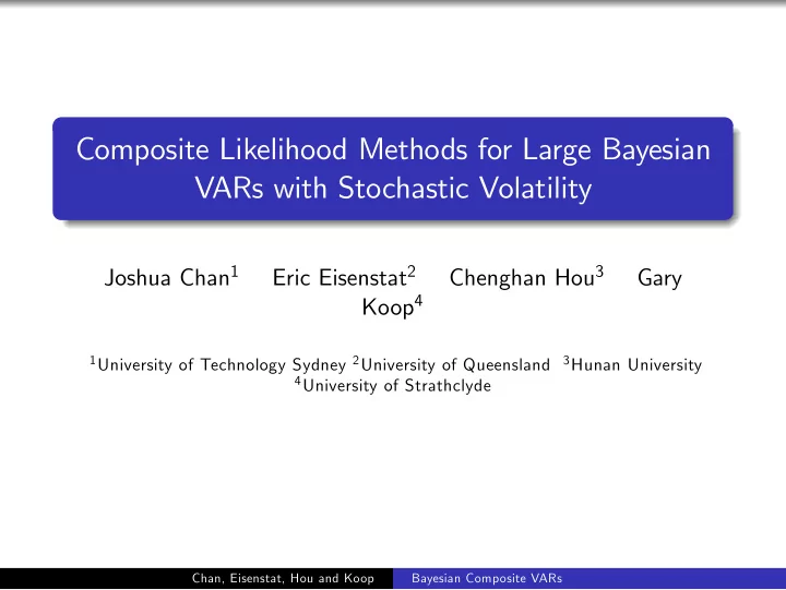
Composite Likelihood Methods for Large Bayesian VARs with Stochastic Volatility Joshua Chan 1 Eric Eisenstat 2 Chenghan Hou 3 Gary Koop 4 1 University of Technology Sydney 2 University of Queensland 3 Hunan University 4 University of Strathclyde

SLIDE 1

Composite Likelihood Methods for Large Bayesian VARs with Stochastic Volatility

Joshua Chan1 Eric Eisenstat2 Chenghan Hou3 Gary Koop4

1University of Technology Sydney 2University of Queensland 3Hunan University 4University of Strathclyde Chan, Eisenstat, Hou and Koop Bayesian Composite VARs

SLIDE 2

Background: History of Large VARs

Large VARs, involving 100 or more dependent variables, are increasingly used in a variety of macroeconomic applications. Pioneering paper: Banbura, Giannone and Reichlin (2010, JAE) "Large Bayesian Vector Autoregressions” Previous VARs: a few variables perhaps 10 at most BGR has 131 variables (standard US macro variables) Many others, here is a sample: Carriero, Kapetanios and Marcellino (2009, IJF): exchange rates for many countries Carriero, Kapetanios and Marcellino (2012, JBF): US government bond yields of different maturities Giannone, Lenza, Momferatou and Onorante (2010): euro area inflation forecasting (components of inflation) Koop and Korobilis (2016, EER) eurozone sovereign debt crisis Bloor and Matheson (2010, EE): macro application for New Zealand Jaroci´ nski and Ma´ ckowiak (2016, ReStat): Granger causality Banbura, Giannone and Lenza (2014, ECB): conditional

Chan, Eisenstat, Hou and Koop Bayesian Composite VARs

SLIDE 3

Background: Why large VARs?

Availability of more data More data means more information, makes sense to include it Concerns about missing out important information (omitted variables bias, fundamentalness, etc.) The main alternatives are factor models Principal components squeeze information in large number of variables to small number of factors But this squeezing is done without reference to explanatory power (i.e. squeeze first then put in regression model or VAR): “unsupervised” Large VAR methods are supervised and can easily see role of individual variables And they work: often beating factor methods in forecasting competitions

Chan, Eisenstat, Hou and Koop Bayesian Composite VARs

SLIDE 4

Background: Computation in large VARs

E.g. large VAR with N = 100 variables and a lag length of p = 13: 100, 000+ VAR coefficients 5, 050 free parameters in error covariance. Bayesian prior shrinkage surmounts over-parameterization Standard choices exist: e.g. Minnesota prior Key point 1: Standard approaches are conjugate: analytical results exist (estimation and forecasting — no MCMC needed) Key point 2: Huge posterior covariance of VAR coefficients (N2p × N2p matrix): tough computation Key point 3: Conjugacy greatly simplifies: separately manipulate N × N and Np × Np matrices Key point 4: Using more realistic priors or extending model (e.g. to relax homoskedasticity assumption) loses conjugacy and, thus, computational feasibility Bottom line: Great tools exist for large homoskedastic Bayesian VARs with a particular prior, but cannot easily extend

Chan, Eisenstat, Hou and Koop Bayesian Composite VARs

SLIDE 5

Background: Multivariate Stochastic Volatility in VARs

Allowing for error variances to change in macroeconomic VARs important E.g. Primiceri (2005, ReStud), Sims and Zha (2006, AER), Clark (2011, JBES), etc. Research question: How to add multivariate stochastic volatility in large VARs? Existing Bayesian literature is either: Homoskedastic Restrictive forms (e.g. Clark, Carriero and Marcellino, 2016, JBES + 2 working papers, Chan, 2016, working paper) Approximations (Koop and Korobilis, JOE, JOE and Koop, Korobilis and Pettenuzzo, 2016, JOE) Present paper: new approach using composite likelihoods

Chan, Eisenstat, Hou and Koop Bayesian Composite VARs

SLIDE 6

Vector Autoregressions with Stochastic Volatility (VAR-SV)

yt is N-vector of dependent variables (N large) VAR-SV is: A0tyt = c + A1yt−1 + · · · Apyt−p + t, t ∼ N(0, Σt), Σt = diag

eh1,t, . . . , ehn,t

A0t =      1 · · · a21,t 1 · · · . . . . . . ... . . . an1,t an2,t · · · 1      Rewrite as yt = Xtβ + Wtat + t Xt = In ⊗ (1, y

t−1, . . . , y t−p)

at is vector of free elements of A0t

Chan, Eisenstat, Hou and Koop Bayesian Composite VARs

SLIDE 7

Vector Autoregressions with Stochastic Volatility

Wt =        · · · · · · · · · −y1,t · · · · · · · · · −y1,t −y2,t · · · · · · · · · . . . . . . ... . . . · · · · · · · · · · · · −y1,t −y2,t · · · −yN−1,t        ht = ht−1 + h

t ,

h

t ∼ N(0, Σh)

at = at−1 + a

t ,

a

t ∼ N(0, Σa)

Σh = diag(σ2

h,1, . . . , σ2 h,N) and Σa = diag(σ2 a,1, . . . , σ2 a, N(N−1)

). Standard MCMC methods used for estimation and forecasting But these will not work with large VARs

Chan, Eisenstat, Hou and Koop Bayesian Composite VARs

SLIDE 8

Composite Bayesian Methods

Likelihood function (assuming independent errors): L (y; θ) =

T

p (yt|θ) =

T

L (yt; θ) Composite likelihood LC (y; θ) =

T

M

LC (yi,t; θ)wi yi,t for i = 1, .., M are sub-vectors of yt LC (yi,t; θ) = p (yi,t|θ) wi weight attached to sub-model i M

i=1 wi = 1

Bayesian composite posterior pC (θ|y) ∝ LC (y; θ) p (θ)

Chan, Eisenstat, Hou and Koop Bayesian Composite VARs

SLIDE 9

How do we use composite Bayesian methods?

Instead of forecasting with large VAR-SV, forecast with many small VAR-SVs Let yt = y∗

t

zt

y∗

t contains N∗ variables of interest

zt (with elements denoted by zi,t) remaining variables. Sub-model i is VAR-SV using yi,t = y∗

t

zi,t

Our application uses 193 variables with N∗ = 3

Thus, 190 sub-models, each is a 4-variate VAR-SV

Chan, Eisenstat, Hou and Koop Bayesian Composite VARs

SLIDE 10

Theory of Composite Likelihood Methods

Some asymptotic theory exists (e.g. Canova and Matthes, 2017) Require strong assumptions Overview: Varin, Reid and Firth (2011, Stat Sin) Pakel, Shephard, Sheppard and Engle (2014, working paper) Need asymptotic mixing assumptions about dependence over time, over variables and between different variables at different points in time In general, strong assumptions often not achieved in practice Hence, our justification is mostly empirical

Chan, Eisenstat, Hou and Koop Bayesian Composite VARs

SLIDE 11

Theory of Composite Likelihoods as Opinion Pools

Bayesian theory uses idea of opinion pool Each sub-model is “agent” with “opinion” about a feature (e.g. a forecast) expressed through a probability distribution. Theory addresses “How do we combine these opinions?” Generalized logarithmic opinion pool equivalent to composite likelihood Nice properties (e.g. external Bayesianity) Linear opinion pools lead to other combinations of sub-models E.g. Geweke and Amisano (2011, JOE) optimal prediction pools In empirical work consider both composite likelihood and Geweke-Amisano

Chan, Eisenstat, Hou and Koop Bayesian Composite VARs

SLIDE 12

Choosing the Weights

Various approaches considered Equal weights wi = 1

M

Weights proportional to marginal likelihood of each sub-model Weights proportional to (exponential of) BIC of each sub-model Weights proportional to (exponential of) DIC of each sub-model In all above use likelihood/marginal likelihood for core variables only (y∗

t )

Chan, Eisenstat, Hou and Koop Bayesian Composite VARs

SLIDE 13

Computation

Target: Draws from Bayesian composite posterior pC (θ|y) ∝ LC (y; θ) p (θ) We have:

1. MCMC draws from M sub-models (4-variate VAR-SVs)
2. Weights, wi for i = 1, .., M

We develop accept-reject algorithm See paper for details

Chan, Eisenstat, Hou and Koop Bayesian Composite VARs

SLIDE 14

Macroeconomic Forecasting Using a Large Dataset

FRED-QD data set from1959Q1- 2015Q3 193 quarterly US variables (transformed to stationarity) Three core variables: CPI inflation, GDP growth and the Federal Funds rate. Small data set: 7 variables Core variables + unemployment, industrial production, money (M2) and stock prices (S&P) Large data set: All 193 variables Lag length of 4

Chan, Eisenstat, Hou and Koop Bayesian Composite VARs

SLIDE 15

Organization

With small data set use variety of models Computation is feasible (and over-parameterization concerns smaller) Large data set: Compare composite likelihoods methods to homoskedastic, conjugate prior, large VAR

Chan, Eisenstat, Hou and Koop Bayesian Composite VARs

SLIDE 16

Priors

For composite likelihood approach prior elicitation less of an issue (small models) With large VARs prior elicitation is crucial (may or may not be disadvantage) For all models use comparable priors Hyperparameter choices inspired by Minnesota prior See paper for details

Chan, Eisenstat, Hou and Koop Bayesian Composite VARs

SLIDE 17

Models

Variety of different weights in composite likelihood approaches Standard VAR-SV (Primiceri, 2005, ReStud) Homoskedastic VARs of different dimensions Carriero, Clark and Marcellino (CCM, 2016a,b) CCM1: common drifting volatility model VAR-SV with at = 0 and Σt = ehtΣ ht is scalar stochastic volatility process CCM2: more flexible SV model VAR-SV with at constant Each equation error has own volatility, but restrictions on correlations

Chan, Eisenstat, Hou and Koop Bayesian Composite VARs

SLIDE 18

Description VAR-HM 7-variable Homoskedastic VAR VAR-SV 7-variable VAR with stochastic volatility VAR-CCM1 7-variable model of CCM (2016a) VAR-CCM2 7-variable model of CCM (2016b) Large VAR large Homoskedastic VAR VAR-CL-BIC VAR-CL-SV with BIC based weights VAR-CL-DIC VAR-CL-SV with DIC based weights VAR-CL-EQ VAR-CL-SV with equal weights VAR—GA VAR—SV with G-A weights VAR-CL-ML VAR-CL-SV with ML weights

Chan, Eisenstat, Hou and Koop Bayesian Composite VARs

SLIDE 19

Estimating Variances and Covariances

Key variables of interest (common to all models) are σij,t for i, j = 1, 2, 3 Small data set: VAR-SV will probably be closest to “true” specification (most flexible) Evaluate performance relative to VAR-SV VAR-SV in red in following figures Dotted lines in some figures credible intervals (16th-84th percentiles)

Chan, Eisenstat, Hou and Koop Bayesian Composite VARs

SLIDE 20

Estimating Variances and Covariances

1960 1980 2000 2020 0.5 1 1.5 1960 1980 2000 2020

0.1 0.2 1960 1980 2000 2020 0.02 0.04 1960 1980 2000 2020 1 2 1960 1980 2000 2020

0.05

0.05 0.1 1960 1980 2000 2020 0.2 0.4 VAR-SV VAR-CL-ML VAR-CL-EQ VAR-CCM2

Chan, Eisenstat, Hou and Koop Bayesian Composite VARs

SLIDE 21

Comparison of VAR-CL-ML to VAR-SV

1960 1980 2000 2020 0.5 1 1.5 1960 1980 2000 2020

0.2 0.4 1960 1980 2000 2020

0.05

0.05 0.1 1960 1980 2000 2020 1 2 3 1960 1980 2000 2020

0.1 0.2 1960 1980 2000 2020 0.2 0.4 0.6

Chan, Eisenstat, Hou and Koop Bayesian Composite VARs

SLIDE 22

Comparison of VAR-CCM1 to VAR-SV

1960 1980 2000 2020 1 2 1960 1980 2000 2020

0.2 1960 1980 2000 2020

0.1 0.2 1960 1980 2000 2020 2 4 1960 1980 2000 2020

0.1 0.2 1960 1980 2000 2020 0.2 0.4 0.6

Chan, Eisenstat, Hou and Koop Bayesian Composite VARs

SLIDE 23

Comparison of VAR-CCM2 to VAR-SV

1960 1980 2000 2020 0.5 1 1.5 1960 1980 2000 2020

0.1 0.2 1960 1980 2000 2020

0.05

0.05 0.1 1960 1980 2000 2020 1 2 1960 1980 2000 2020

0.05

0.05 0.1 1960 1980 2000 2020 0.2 0.4 0.6

Chan, Eisenstat, Hou and Koop Bayesian Composite VARs

SLIDE 24

Comparison of VAR-HM to VAR-SV

1960 1980 2000 2020 0.5 1 1960 1980 2000 2020

0.1 0.2 1960 1980 2000 2020

0.02

0.02 0.04 0.06 1960 1980 2000 2020 0.5 1 1.5 1960 1980 2000 2020

0.05

0.05 0.1 1960 1980 2000 2020 0.1 0.2 0.3

Chan, Eisenstat, Hou and Koop Bayesian Composite VARs

SLIDE 25

Forecasting

Estimation results are encouraging, what about forecasting? Results for h = 1 Two forecast evaluation periods: Beginning 1970Q1 Beginning 2008Q1 (financial crisis and subsequent recession)

Chan, Eisenstat, Hou and Koop Bayesian Composite VARs

SLIDE 26

Forecast Evaluation Metrics

For 3 core variables individually: RMSFE MAFE ALPL = average of log predictive likelihoods (higher value better) ACRPS = average of conditional rank probability score (lower values better) Also joint ALPL based on joint predictive for core variables

Chan, Eisenstat, Hou and Koop Bayesian Composite VARs

SLIDE 27

Joint ALPL for Core Variables

Forecast Performance Post-1970 Post-2008 VAR-HM 0.33 −0.58 VAR-SV 0.65 0.44 VAR-CCM1 0.06 −0.51 VAR-CCM2 0.90 0.52 Large VAR −0.47 −1.69 VAR-CL-ML 0.90 1.27 VAR-CL-DIC 0.85 0.67 VAR-CL-BIC 0.90 1.15 VAR-CL-EQ 0.88 0.89 VAR-GA 0.91 1.01

Chan, Eisenstat, Hou and Koop Bayesian Composite VARs

SLIDE 28

Joint ALPL for Core Variables

Best overall summary Composite likelihoods + Geweke-Amisano forecast best Weights: Marginal likelihood or BIC weights best (but only slightly) Homoskedastic large VAR does poorly CCM2 better than CCM1

Chan, Eisenstat, Hou and Koop Bayesian Composite VARs

SLIDE 29

Forecasting the Core Forecasts Individually

Following tables present results for each variable General themes: Composite likelihoods+GA forecast well Especially for 2008-2016 period Especially for inflation and interest rate Less so for GDP growth (VAR-SV is best) Large homoskedastic VARs forecast poorly CCM2 better than CCM1 In general, CCM2 similar but a bit worse than composite likelihoods

Chan, Eisenstat, Hou and Koop Bayesian Composite VARs

SLIDE 30

Inflation Forecasting Beginning in 1970

RMSFE MAE ACRPS ALPL VAR-HM 0.66 0.45 0.36 −0.15 VAR-SV 0.67 0.46 0.36 −0.06 VAR-CCM1 0.71 0.51 0.39 −0.12 VAR-CCM2 0.67 0.46 0.36 −0.00 Large VAR 0.73 0.52 0.56 −0.14 VAR-CL-ML 0.69 0.47 0.36 −0.01 VAR-CL-DIC 0.68 0.47 0.36 −0.01 VAR-CL-BIC 0.69 0.46 0.36 −0.01 VAR-CL-EQ 0.68 0.47 0.36 −0.01 VAR-GA 0.68 0.47 0.38 −0.00

Chan, Eisenstat, Hou and Koop Bayesian Composite VARs

SLIDE 31

Inflation Forecasting Beginning in 2008

RMSFE MAE ACRPS ALPL VAR-HM 1.04 0.66 0.52 −1.16 VAR-SV 1.06 0.68 0.54 −0.68 VAR-CCM1 1.04 0.66 0.52 −0.71 VAR-CCM2 1.05 0.68 0.53 −0.57 Large VAR 1.03 0.65 0.69 −0.71 VAR-CL-ML 1.04 0.65 0.51 −0.54 VAR-CL-DIC 1.04 0.66 0.52 −0.57 VAR-CL-BIC 1.02 0.63 0.50 −0.50 VAR-CL-EQ 1.04 0.66 0.52 −0.57 VAR-GA 1.03 0.66 0.54 −0.48

Chan, Eisenstat, Hou and Koop Bayesian Composite VARs

SLIDE 32

Interest Rate Forecasting Beginning in 1970

RMSFE MAE ACRPS ALPL VAR-HM 0.29 0.18 0.15 0.81 VAR-SV 0.28 0.17 0.14 1.03 VAR-CCM1 0.51 0.33 0.25 0.53 VAR-CCM2 0.28 0.17 0.14 1.19 Large VAR 0.56 0.42 0.44 0.17 VAR-CL-ML 0.28 0.17 0.13 1.18 VAR-CL-DIC 0.28 0.16 0.13 1.17 VAR-CL-BIC 0.28 0.17 0.13 1.20 VAR-CL-EQ 0.27 0.16 0.13 1.19 VAR-GA 0.27 0.16 0.13 1.21

Chan, Eisenstat, Hou and Koop Bayesian Composite VARs

SLIDE 33

Interest Rate Forecasting Beginning in 2008

RMSFE MAE ACRPS ALPL VAR-HM 0.25 0.18 0.14 0.97 VAR-SV 0.18 0.12 0.10 1.50 VAR-CCM1 0.36 0.30 0.20 0.66 VAR-CCM2 0.20 0.12 0.10 1.45 Large VAR 0.51 0.45 0.46 0.09 VAR-CL-ML 0.13 0.07 0.06 2.00 VAR-CL-DIC 0.13 0.08 0.07 1.67 VAR-CL-BIC 0.13 0.07 0.06 1.88 VAR-CL-EQ 0.12 0.08 0.07 1.79 VAR-GA 0.12 0.08 0.07 1.83

Chan, Eisenstat, Hou and Koop Bayesian Composite VARs

SLIDE 34

GDP growth Forecasting Beginning in 1970

RMSFE MAE ACRPS ALPL VAR-HM 0.89 0.68 0.51 −0.38 VAR-SV 0.86 0.65 0.50 −0.32 VAR-CCM1 0.87 0.67 0.51 −0.36 VAR-CCM2 0.86 0.66 0.50 −0.31 Large VAR 0.93 0.70 0.77 −0.39 VAR-CL-ML 0.92 0.67 0.51 −0.35 VAR-CL-DIC 0.91 0.67 0.51 −0.36 VAR-CL-BIC 0.93 0.68 0.52 −0.35 VAR-CL-EQ 0.92 0.68 0.51 −0.35 VAR-GA 0.92 0.68 0.54 −0.36

Chan, Eisenstat, Hou and Koop Bayesian Composite VARs

SLIDE 35

GDP growth Forecasting Beginning in 2008

RMSFE MAE ACRPS ALPL VAR-HM 0.96 0.72 0.56 −0.48 VAR-SV 0.86 0.63 0.50 −0.42 VAR-CCM1 0.94 0.73 0.57 −0.57 VAR-CCM2 0.88 0.65 0.52 −0.46 Large VAR 0.96 0.77 0.80 −0.47 VAR-CL-ML 0.95 0.65 0.52 −0.46 VAR-CL-DIC 0.95 0.66 0.53 −0.50 VAR-CL-BIC 0.96 0.67 0.52 −0.47 VAR-CL-EQ 0.95 0.66 0.52 −0.47 VAR-GA 0.96 0.68 0.56 −0.46

Chan, Eisenstat, Hou and Koop Bayesian Composite VARs

SLIDE 36

Conclusion

Composite likelihood methods allows VAR-SV with huge data sets Computationally and conceptually simple: average over many small models Other VAR-SV models have some attractive features but are computationally infeasible with huge data sets In small data set, composite likelihood methods approximate

ther methods

In large data set, composite likelihoods forecast better than large VAR

Chan, Eisenstat, Hou and Koop Bayesian Composite VARs