Comparison of semi-parametric reduced bias quantile estimators Maria - PowerPoint PPT Presentation

Comparison of semi-parametric reduced bias’ quantile estimators Comparison of semi-parametric reduced bias’ quantile estimators Maria Ivette Gomes (CEAUL and DEIO, Universidade de Lisboa) Fernanda Figueiredo (Universidade do Porto (FEP) and CEAUL) Bjorn Vandewalle (Katholieke Universiteit Leuven and CEAUL) EVA, OSLO 2005

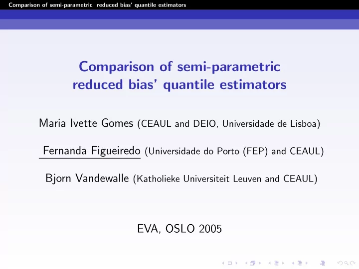
Comparison of semi-parametric reduced bias’ quantile estimators Plan Motivation and Introduction Second Order Reduced Bias’ Tail Index Estimators Asymptotic Behaviour of Reduced Bias’ High Quantile Estimators Simulated Behaviour of High Quantile Estimators Case-study Some Overall Conclusions

Comparison of semi-parametric reduced bias’ quantile estimators 1. Motivation and Introduction Motivation Heavy-tailed models are quite useful in the most diversified areas (insurance, economics, finance, telecommunications, biostatistics,...) and the classical semi-parametric estimators of extreme events’ parameters usually exhibit a reasonably high bias for low thresholds, i.e., for large values of k , the number of top o.s. used for the estimation. Recently, new classes of reduced bias’ tail index estimators have been introduced in the literature. The estimation of the second order parameters in the bias at a level k 1 larger than k , the level at which we compute the tail index estimators, enables keeping the asymptotic variance of the new estimators equal to the asymptotic variance of the Hill estimator, � k H ( k ) := U i / k , U i := i (ln X n − i +1: n − ln X n − i : n ) , 1 ≤ i ≤ k . i =1

Comparison of semi-parametric reduced bias’ quantile estimators 1. Motivation and Introduction Here we deal with bias reduction techniques for heavy tails, trying to improve the performance of the classical high quantile estimators, strongly dependent on the tail index estimation. Main objectives of this presentation: 1 Introduce new classes of high quantiles’ estimators in the lines of Gomes and Figueiredo (2003) and Matthys and Beirlant (2003) 2 Prove their consistency and asymptotic normality under appropriate conditions 3 Compare them with alternative ones through Monte Carlo simulations

Comparison of semi-parametric reduced bias’ quantile estimators 1. Motivation and Introduction Introduction Definition 1: A model F is said to have a heavy right tail whenever the maximum, linearly normalized, of an i.i.d. sample of size n , converges weakly, as n → ∞ , towards the Extreme Value d.f., � � − (1 + γ x ) − 1 /γ � exp , 1 + γ x > 0 if γ � = 0 EV γ ( x ) = γ = 0 , exp( − exp( − x )) , x ∈ R if with γ > 0. We write F ∈ D M ( EV γ ), with D M denoting domain of attraction for maxima. Let RV α denote the class of regularly varying functions with index α , i.e., positive measurable functions g such that t →∞ g ( tx ) / g ( t ) = x α , for all x > 0. lim For γ > 0, U ( t ) := F ← (1 − 1 / t ) = inf { x : F ( x ) ≥ 1 − 1 / t } and F ← the generalized inverse of the underlying model F , F ∈ D M ( EV γ ) ⇔ 1 − F ∈ RV − 1 /γ ⇔ U ∈ RV γ .

Comparison of semi-parametric reduced bias’ quantile estimators 1. Motivation and Introduction Main objective of this paper: Estimate a value χ p such that 1 − F ( χ p ) = p , with p small, more specifically, χ p = U (1 / p ) , p = p n → 0 , n p n → K , as n → ∞ , 0 ≤ K ≤ 1 . We shall assume to be working in Hall’s class of models, where there exist γ > 0, ρ < 0, C > 0 and β � = 0 such that U ( t ) = Ct γ � � 1 + γ β t ρ + o ( t ρ ) , as t → ∞ . ρ We are going to base inference on the largest k top o.s., i.e., we shall assume k to be intermediate , k = k n → ∞ , k = o ( n ) as n → ∞ . Possible semi-parametric quantile estimator: � k � ❜ γ Q ( p ) γ ( k ) := X n − k : n ( Weissman , 1978) . ❜ np

Comparison of semi-parametric reduced bias’ quantile estimators 1. Motivation and Introduction Classical quantile estimator: P k � k � � k � H ( k ) U i / k Q ( p ) i =1 H ( k ) := X n − k : n =: X n − k : n . np np To derive the asymptotic non-degenerate behaviour of the semi-parametric estimators, we assume = x ρ − 1 ln U ( tx ) − ln U ( t ) − γ ln x lim , for all x > 0 , A ( t ) ρ t →∞ where A ( · ) is a function of constant sign near infinity, ρ ≤ 0 is the second order parameter and | A | ∈ RV ρ (Geluk and de Haan, 1987). We assume ρ < 0, and since we are working with models in Hall’s class, the previous second order condition holds true with A ( t ) = γ β t ρ , and for an adequate k , we may guarantee the asymptotic normality of the Hill estimator.

Comparison of semi-parametric reduced bias’ quantile estimators 1. Motivation and Introduction Proposition 1 [de Haan and Peng, 1998]: We may write the asymptotic distributional representation k � H ( k ) := 1 = γ + γ P k + A ( n / k ) d U i √ 1 − ρ (1 + o p (1)) , k k i =1 �� k � √ P k = i =1 E i / k − 1 , with { E i } standard exponential i.i.d. k r.v.’s. Consequently, if we choose a level k such that √ √ k A ( n / k ) → λ � = 0, finite, as n → ∞ , k ( H ( k ) − γ ) is asymptotically normal, with a non-null bias given by λ/ (1 − ρ ). Most of the times, this type of estimates exhibit a strong bias for moderate k and sample paths with very short stability regions around the target value γ . This problem has been recently addressed by several authors, who consider the possibility of dealing with the bias term in an appropriate way, building different new estimators, � γ R ( k ) say, the so-called second order reduced bias’ estimators.

Comparison of semi-parametric reduced bias’ quantile estimators 2. Second Order Reduced Bias’ Tail Index Estimators Second Order Reduced Bias’ Tail Index Estimators Definition 2: A tail index estimator � γ R ( k ) is said to be a second order reduced bias’ estimator if, for k intermediate, and under the second order framework, we may write R = γ + σ R P d k � γ R ( k ) √ + o p ( A ( n / k )) , k R with P k an asymptotically standard normal r.v., σ R > 0 and A ( · ) being again the function controlling the speed of convergence of maximum values, linearly normalized, towards a non-degenerate r.v. with d.f. EV γ . √ Remark 1: k ( � γ R ( k ) − γ ) is asymptotically normal with a null √ mean value even when k A ( n / k ) → λ , finite, possibly non-null, as n → ∞ .

Comparison of semi-parametric reduced bias’ quantile estimators 2. Second Order Reduced Bias’ Tail Index Estimators Gomes and Figueiredo (2003) suggest the use of reduced bias’ tail index estimators in the quantile estimator functional expression, in order to reduce also the dominant component of the classical quantile estimator’s asymptotic bias. Mathys and Beirlant (2003) try also to reduce the bias of the classical quantile estimators, going directly into the second order framework. With Y i : n , 1 ≤ i ≤ n , denoting the set of ascending o.s. associated to a standard Pareto i.i.d. sample, � � 1 + A ( n / k ) a ρ χ p U (1 / p ) n − 1 p ∼ a γ = , a n = k / ( n p n ) . n U ( Y n − k : n ) ρ X n − k : n γ, � For A ( t ) = γ β t ρ , ( � β, � ρ ) a suitable estimator of ( γ, β, ρ ), they get � k � ❜ � � � n � ❜ γ ρ − 1 ρ ( k / ( np )) ❜ ( p ) γ � Q γ ( k ) := X n − k : n exp � β . ❜ np k � ρ

Comparison of semi-parametric reduced bias’ quantile estimators 2. Second Order Reduced Bias’ Tail Index Estimators It is known ( Gomes and Figueiredo, 2003 ) that the use of a reduced bias’ tail index estimator � γ R provides better results than the use of the classical Hill estimator H . The obvious question that we shall try to answer both theoretically and computationally, is the following: Is it better to work with 1 the estimator Q ( p ) and a reduced bias estimator � γ ≡ � γ R γ ❜ of γ , ( p ) 2 the estimator Q and a classical estimator of γ , like the ❜ γ Hill estimator H ( k ), ( p ) 3 or the estimator Q and a reduced bias estimator � γ R of γ ❜ γ ?

Comparison of semi-parametric reduced bias’ quantile estimators 2. Second Order Reduced Bias’ Tail Index Estimators We shall use the second order reduced bias’ tail index estimator from Gomes and Martins (2002). With the notation � i � − ρ k � � i � − ρ U i , s ρ ( k ) = 1 � k and S ρ ( k ) = 1 i =1 k k k k i =1 we may write the “maximum likelihood” estimator for the tail index γ in the form ρ ( k ) S 0 ( k ) − S ❜ ρ ( k ) ρ ( k ) × s ❜ M ( k ) ≡ M ❜ ρ ( k ) := S 0 ( k ) − S ❜ ρ ( k ) . s ❜ ρ ( k ) S ❜ ρ ( k ) − S 2 ❜ Remark 2: This estimator attains the minimal asymptotic variance in Drees’ class of functionals (Drees, 1998), given by ( γ (1 − ρ ) /ρ ) 2 .