QUANTILE AUTOREGRESSION ROGER KOENKER AND ZHIJIE XIAO Abstract. We - - PDF document

SLIDE 1

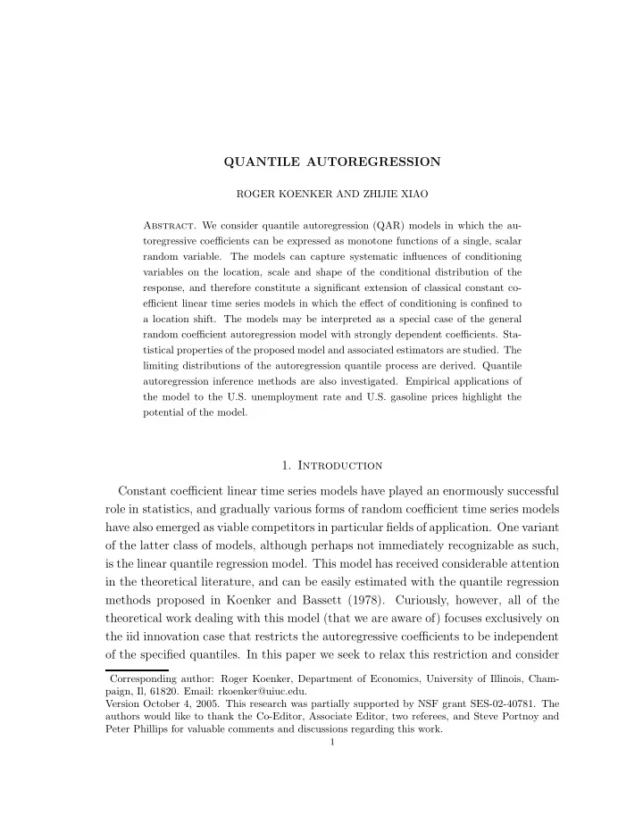
QUANTILE AUTOREGRESSION

ROGER KOENKER AND ZHIJIE XIAO

• Abstract. We consider quantile autoregression (QAR) models in which the au-

toregressive coefficients can be expressed as monotone functions of a single, scalar random variable. The models can capture systematic influences of conditioning variables on the location, scale and shape of the conditional distribution of the response, and therefore constitute a significant extension of classical constant co- efficient linear time series models in which the effect of conditioning is confined to a location shift. The models may be interpreted as a special case of the general random coefficient autoregression model with strongly dependent coefficients. Sta- tistical properties of the proposed model and associated estimators are studied. The limiting distributions of the autoregression quantile process are derived. Quantile autoregression inference methods are also investigated. Empirical applications of the model to the U.S. unemployment rate and U.S. gasoline prices highlight the potential of the model.

• 1. Introduction

Constant coefficient linear time series models have played an enormously successful role in statistics, and gradually various forms of random coefficient time series models have also emerged as viable competitors in particular fields of application. One variant

• f the latter class of models, although perhaps not immediately recognizable as such,

is the linear quantile regression model. This model has received considerable attention in the theoretical literature, and can be easily estimated with the quantile regression methods proposed in Koenker and Bassett (1978). Curiously, however, all of the theoretical work dealing with this model (that we are aware of) focuses exclusively on the iid innovation case that restricts the autoregressive coefficients to be independent

• f the specified quantiles. In this paper we seek to relax this restriction and consider

Corresponding author: Roger Koenker, Department of Economics, University of Illinois, Cham- paign, Il, 61820. Email: rkoenker@uiuc.edu. Version October 4, 2005. This research was partially supported by NSF grant SES-02-40781. The authors would like to thank the Co-Editor, Associate Editor, two referees, and Steve Portnoy and Peter Phillips for valuable comments and discussions regarding this work.

1

SLIDE 2

2 Quantile Autoregression

linear quantile autoregression models whose autoregressive (slope) parameters may vary with quantiles τ ∈ [0, 1]. We hope that these models might expand the modeling

• ptions for time series that display asymmetric dynamics or local persistency.

Considerable recent research effort has been devoted to modifications of traditional constant coefficient dynamic models to incorporate a variety of heterogeneous inno- vation effects. An important motivation for such modifications is the introduction of asymmetries into model dynamics. It is widely acknowledged that many important economic variables may display asymmetric adjustment paths (e.g. Neftci (1984), Enders and Granger (1998)). The observation that firms are more apt to increase than to reduce prices is a key feature of many macroeconomic models. Beaudry and Koop (1993) have argued that positive shocks to U.S. GDP are more persistent than negative shocks, indicating asymmetric business cycle dynamics over different quantiles of the innovation process. In addition, while it is generally recognized that

• utput fluctuations are persistent, less persistent results are also found at longer hori-

zons (Beaudry and Koop (1993)), suggesting some form of “local persistency.” See, inter alia, Delong and Summers (1986), Hamilton (1989), Evans and Wachtel (1993), Bradley and Jansen (1997), Hess and Iwata (1997), and Kuan and Huang (2001). A related development is the growing literature on threshold autoregression (TAR) see e.g. Balke and Fomby (1997); Tsay (1997); Gonzalez and Gonzalo (1998); Hansen (2000); and Caner and Hansen (2001). We believe that quantile regression methods can provide an alternative way to study asymmetric dynamics and local persistency in time series. We propose a new quantile autoregression (QAR) model in which autoregressive coefficients may take distinct values over different quantiles of the innovation process. We show that some forms of the model can exhibit unit-root-like tendencies or even temporarily explosive behavior, but occasional episodes of mean reversion are sufficient to insure stationar-

• ity. The models lead to interesting new hypotheses and inference apparatus for time

series. The paper is organized as follows: We introduce the model and study some basic statistical properties of the QAR process in Section 2. Section 3 develops the limiting distribution of the QAR estimator. Section 4 considers some restrictions imposed

• n the model by the monotonicity requirement on the conditional quantile functions.

Statistical inference, including testing for asymmetric dynamics, is explored in Section

SLIDE 3

Roger Koenker and Zhijie Xiao 3

• 5. Section 6 reports a Monte Carlo experiment on the sampling performance of the

proposed inference procedure. An empirical application to U.S. unemployment rate time series is given in Section 7. Proofs appear in the Appendix.

• 2. The Model

There is a substantial theoretical literature, including Weiss (1987), Knight (1989), Koul and Saleh(1995), Koul and Mukherjee(1994), Herc´ e (1996), Hasan and Koenker (1997), Hallin and Jureˇ ckov´ a (1999) dealing with the linear quantile autoregression model. In this model the τ-th conditional quantile function of the response yt is expressed as a linear function of lagged values of the response. The current paper wish to study estimation and inference in a more general class of quantile autoregressive (QAR) models in which all of the autoregressive coefficients are allowed to be τ- dependent, and therefore are capable of altering the location, scale and shape of the conditional densities. 2.1. The Model. Let {Ut} be a sequence of iid standard uniform random variables, and consider the pth order autoregressive process, (1) yt = θ0(Ut) + θ1(Ut)yt−1 + · · · + θp(Ut)yt−p, where the θj’s are unknown functions [0, 1] → R that we will want to estimate. Provided that the right hand side of (1) is monotone increasing in Ut, it follows that the τth conditional quantile function of yt can be written as, (2) Qyt(τ|yt−1, ..., yt−p) = θ0(τ) + θ1(τ)yt−1 + ... + θp(τ)yt−p,

• r somewhat more compactly as,

(3) Qyt(τ|Ft−1) = x⊤

t θ(τ).

where xt = (1, yt−1, ..., yt−p)⊤, and Ft is the σ-field generated by {ys, s ≤ t}. The tran- sition from (1) to (2) is an immediate consequence of the fact that for any monotone increasing function g and standard uniform random variable, U, we have Qg(U)(τ) = g(QU(τ)) = g(τ), where QU(τ) = τ is the quantile function of U. In the above model, the autore- gressive coefficients may be τ-dependent and thus can vary over the quantiles. The conditioning variables not only shift the location of the distribution of yt, but also

SLIDE 4

4 Quantile Autoregression

may alter the scale and shape of the conditional distribution. We will refer to this model as the QAR(p) model. We will argue that QAR models can play a useful role in expanding the modeling territory between classical stationary linear time series models and their unit root

• alternatives. To illustrate this in the QAR(1) case, consider the model

(4) Qyt(τ|Ft−1) = θ0(τ) + θ1(τ)yt−1, with θ0(τ) = σΦ−1(τ), and θ1(τ) = min{γ0 + γ1τ, 1} for γ0 ∈ (0, 1) and γ1 > 0. In this model if Ut > (1 − γ0)/γ1 the model generates the yt according to the standard Gaussian unit root model, but for smaller realizations of Ut we have a mean reversion

• tendency. Thus, the model exhibits a form of asymmetric persistence in the sense that

sequences of strongly positive innovations tend to reinforce its unit root like behavior, while occasional negative realizations induce mean reversion and thus undermine the persistence of the process. The classical Gaussian AR(1) model is obtained by setting θ1(τ) to a constant. The formulation in (4) reveals that the model may be interpreted as somewhat special form of random coefficient autoregressive (RCAR) model. Such models arise naturally in many time series applications. Discussions of the role of RCAR models can be found in, inter alia, Nicholls and Quinn (1982), Tjøstheim(1986), Pourahmadi (1986), Brandt (1986), Karlsen(1990), and Tong (1990). In contrast to most of the literature on RCAR models, in which the coefficients are typically assumed to be stochastically independent of one another, the QAR model has coefficients that are functionally dependent. Monotonicity of the conditional quantile functions imposes some discipline on the forms taken by the θ functions. This discipline essentially requires that the function Qyt(τ|yt−1, ..., yt−p) is monotone in τ in some relevant region Υ of (yt−1, ..., yt−p)-space. The correspondance between the random coefficient formulation of the QAR model (1) and the conditional quantile function formulation (2) presupposes the monotonicity

• f the latter in τ. In the region Υ where this monotonicity holds (1) can be regarded

as a valid mechanism for simulating from the QAR model (2). Of course, model (1) can, even in the absence of this monotonicity, be taken as a valid data generating mechanism, however the link to the strictly linear conditional quantile model is no longer valid. At points where the monotonicity is violated the conditional quantile

SLIDE 5

Roger Koenker and Zhijie Xiao 5

functions corresponding to the model described by (1) have linear “kinks”. Attempt- ing to fit such piecewise linear models with linear specifications can be hazardous. We will return to this issue in the discussion of Section 4. In the next section we briefly describe some essential features of the QAR model. 2.2. Properties of the QAR Process. The QAR(p) model (1) can be reformulated in more conventional random coefficient notation as, (5) yt = µ0 + α1,tyt−1 + · · · + αp,tyt−p + ut where µ0 = Eθ0(Ut), ut = θ0(Ut)−µ0, and αj,t = θj(Ut), for j = 1, ..., p. Thus, {ut} is an iid sequence of random variables with distribution function F(·) = θ−1

0 (·+µ0), and

the αj,t coefficients are functions of this ut innovation random variable. The QAR(p) process (5) can be expressed as an p-dimensional vector autoregression process of

• rder 1:

Yt = Γ + AtYt−1 + Vt with Γ =

• µ0

0p−1

• , At =
• Ap−1,t

αp,t Ip−1 0p−1

• , Vt =
• ut

0p−1

• ,

where Ap−1,t = [ α1,t, . . . , αp−1,t ], Yt = [yt, · · ··, yt−p+1]⊤, and 0p−1 is the (p − 1)- dimensional vector of zeros. In the Appendix, we show that under regularity condi- tions given in the following Theorem, an Ft-measurable solution for (5) can be found. To formalize the foregoing discussion and facilitate later asymptotic analysis, we introduce the following conditions. A.1: {ut} are iid random variables with mean 0 and variance σ2 < ∞. The distribution function of ut, F, has a continuous density f with f(u) > 0 on U = {u : 0 < F(u) < 1}. A.2: Let E(At ⊗ At) = ΩA, the eigenvalues of ΩA have moduli less than unity. A.3: Denote the conditional distribution function Pr[yt < ·|Ft−1] as Ft−1(·) and its derivative as ft−1(·), ft−1 is uniformly integrable on U.

SLIDE 6

6 Quantile Autoregression

Theorem 2.1. Under assumptions A.1 and A.2, the time series yt given by (5) is covariance stationary and satisfies a central limit theorem 1 √n

n

• t=1

(yt − µy) ⇒ N

• 0, ω2

y

• ,

where µy = µ0/(1 − p

j=1 µj), ω2 y = lim n−1E[n t=1(yt − µy)]2, and µj = E(αj,t), j =

1, ..., p. To illustrate some important features of the QAR process, we consider the simplest case of QAR(1) process, (6) yt = αtyt−1 + ut, where αt = θ1(Ut) and ut = θ0(Ut) corresponding to (4), whose properties are sum- marized in the following corollary. Corollary 2.1. If yt is determined by (6), and ω2

α = E(αt)2 < 1, under assumption

A.1, yt is covariance stationary and satisfies a central limit theorem 1 √n

n

• t=1

yt ⇒ N

• 0, ω2

y

• ,

where ω2

y = σ2(1 + µα)/((1 − µα)(1 − ω2 α)) with µα = E(αt) < 1.

In the example given in Section 2.1, αt = θ1(Ut) = min{γ0 + γ1Ut, 1} ≤ 1, and Pr (|αt| < 1) > 0, the condition of Corollary 2.1 holds and the process yt is globally stationary but can still display local (and asymmetric) persistency in the presence of certain type of shocks (positive shocks in the example). Corollary 2.1 also indicates that even with αt > 1 over some range of quantiles, as long as ω2

α = E(αt)2 < 1,

yt can still be covariance stationary in the long run. Thus, a quantile autoregressive process may allow for some (transient) forms of explosive behavior while maintaining stationarity in the long run. Under the assumptions in Corollary 2.1, by recursively substituting in (6), we can see that (7) yt =

∞

• j=0

βt,jut−j, where βt,0 = 1, and βt,j =

j−1

• i=0

αt−i, for j ≥ 1, is a stationary Ft-measurable solution to (6). In addition, if ∞

j=0 βt,jvt−j converges

in Lp, then yt has a finite p-th order moment. The Ft-measurable solution of (6) gives

SLIDE 7

Roger Koenker and Zhijie Xiao 7

a doubly stochastic MA(∞) representation of yt. In particular, the impulse response

• f yt to a shock ut−j is stochastic and is given by βt,j. On the other hand, although the

impulse response of the quantile autoregressive process is stochastic, it does converge (to zero) in mean square (and thus in probability) as j → ∞, corroborating the stationarity of yt. If we denote the autocovariance function of yt by γy(h), it is easy to verify that γy(h) = µ|h|

α σ2 y where σ2 y = σ2/(1 − ω2 α).

Remark 2.1. Comparing to the QAR(1) process yt, if we consider a conventional AR(1) process with autoregressive coefficient µα and denote the corresponding process by yt, the long-run variance of yt (given by ω2

y) is (as expected) larger than that of

• yt. The additional variance the QAR process yt comes from the variation of αt. In

fact, ω2

y can be decomposed into the summation of the long-run variance of yt and an

additional term that is determined by the variance of αt: ω2

y = ω2 y +

σ2 (1 − µα)2(1 − ω2

α)Var(αt),

where ω2

y = σ2/(1 − µα)2 is the long-run variance of yt.

We consider estimation and related inference on the QAR model in the next two sections.

• 3. Estimation

Estimation of the quantile autoregressive model (3) involves solving the problem (8) min

θ∈Rp+1 n

• t=1

ρτ(yt − x⊤

t θ),

where ρτ(u) = u(τ −I(u < 0)) as in Koenker and Bassett (1978). Solutions, θ(τ), are called autoregression quantiles. Given θ(τ), the τ-th conditional quantile function of yt, conditional on xt, could be estimated by, ˆ Qyt(τ|xt) = x⊤

t

θ(τ), and the conditional density of yt can be estimated by the difference quotients, ˆ fyt(τ|xt−1) = (τi − τi−1)/( ˆ Qyt(τi|xt−1) − ˆ Qyt(τi−1|xt−1)), for some appropriately chosen sequence of τ’s.

SLIDE 8

8 Quantile Autoregression

If we denote E(yt) as µy, E(ytyt−j) as γj, and let Ω0 = E(xtx⊤

t ) = lim n−1 n t=1 xtx⊤ t ,

then Ω0 =

• 1

µ⊤

y

µy Ωy

• where µy = µy · 1p×1, and

Ωy =    γ0 · · · γp−1 . . . ... . . . γp−1 · · · γ0    . In the special case of QAR(1) model (6), Ω0 = E(xtx⊤

t ) = diag[1, γ0], γ0 = E[y2 t ].

Let Ω1 = lim n−1 n

t=1 ft−1[F −1 t−1(τ)]xtx⊤ t , and define Σ = Ω−1 1 Ω0Ω−1 1 . The asymptotic

distribution of θ(τ) is summarized in the following Theorem. Theorem 3.1. Under assumptions A.1 - A.3, Σ−1/2√n( θ(τ) − θ(τ)) ⇒ Bk(τ), where Bk(τ) represents a k-dimensional standard Brownian Bridge, k = p + 1. By definition, for any fixed τ, Bk(τ) is N (0, τ(1 − τ)Ik). In the important special case with constant coefficients, Ω1 = f[F −1(τ)]Ω0, where f(·) and F(·) are the density and distribution functions of ut, respectively. We state this result in the following corollary. Corollary 3.1. Under assumptions A.1 - A.3, if the coefficients αjt are constants, then f[F −1(τ)]Ω1/2 √n( θ(τ) − θ(τ)) ⇒ Bk(τ). An alternative form of the model that is widely used in economic applications is the augmented Dickey-Fuller (ADF) regression (9) yt = µ0 + δ0,tyt−1 +

p−1

• j=1

δj,t∆yt−j + ut, where, corresponding to (5), δ0,t =

p

• s=1

αs,t, δj,t = −

p

• s=j+1

αs,t, j = 1, · · ·, p − 1.

SLIDE 9

Roger Koenker and Zhijie Xiao 9

In the above transformed model, δ0,t is the critical parameter corresponding the largest autoregressive root. Let zt = (1, yt−1, ∆yt−1, ..., ∆yt−p+1)⊤, we may write the quantile regression counterpart of (9) as (10) Qyt(τ|Ft−1) = z⊤

t δ(τ),

where δ(τ) = (α0(τ), δ0(τ), δ1(τ), · · ·, δp−1(τ))⊤. The limiting distributions of the quantile regression estimators δ(τ) can be obtained from our previous analysis. If we define J =         1 · · · 1 1 · · · 1 −1 −1 ... · · · −1         , and ∆ = JΣJ, then we have, under assumptions A.1 - A.3, ∆−1/2√n( δ(τ) − δ(τ)) ⇒ Bk(τ). If we focus our attention on the largest autoregressive root δ0,t in the ADF type regression (9) and consider the special case that δj,t = constant for j = 1, ..., p − 1, then, a result similar to Corollary 2.1 can be obtained. Corollary 3.2. Under assumptions A.1-A.3, if δj,t = constant for j = 1, ..., p − 1, and δ0,t ≤ 1 and |δ0,t| < 1 with positive probability, then the time series yt given by (9) is covariance stationary and satisfies a central limit theorem.

• 4. Quantile Monotonicity

As in other linear quantile regression applications, linear QAR models should be cautiously interpreted as useful local approximations to more complex nonlin- ear global models. If we take the linear form of the model too literally then obviously at some point, or points, there will be “crossings” of the conditional quantile func- tions – unless these functions are precisely parallel in which case we are back to the pure location shift form of the model. This crossing problem appears more acute in

SLIDE 10

10 Quantile Autoregression

200 400 600 800 1000 40 80

Figure 1. QAR and Unit Root Time-Series: The figure contrasts two time series generated by the same sequence of innovations. The grey sample path is a random walk with standard Gaussian innovations; the black sample path illustrates a QAR series generated by the same inno- vations with random AR(1) coefficient .85 + .25Φ(ut). The latter series although exhibiting explosive behavior in the upper tail is stationary as described in the text. the autoregressive case than in ordinary regression applications since the support of the design space, i.e. the set of xt that occur with positive probability, is determined within the model. Nevertheless, we may still regard the linear models specified above as valid local approximations over a region of interest. It should be stressed that the estimated conditional quantile functions, ˆ Qy(τ|x) = x⊤ θ(τ), are guaranteed to be monotone at the mean design point, x = ¯ x, as shown in Bassett and Koenker (1982), for linear quantile regression models. In our random coefficient view of the QAR model, yt = x⊤

t θ(Ut),

we express the observable random variable yt as a linear function of conditioning

• covariates. But rather than assuming that the coordinates of the vector θ are inde-

pendent random variables we adopt a diametrically opposite viewpoint – that they are perfectly functionally dependent, all driven by a single random uniform variable. If the functions (θ0, ..., θp) are all monotonically increasing then the coordinates of

SLIDE 11

Roger Koenker and Zhijie Xiao 11

0.2 0.4 0.6 0.8 −1.5 0.0 1.5 tau (Intercept)

• 0.2

0.4 0.6 0.8 0.85 1.00 tau x

• Figure 2. Estimating the QAR model: The figure illustrates estimates
• f the QAR(1) model based on the black time series of the previous
• figure. The left panel represents the intercept estimate at 19 equally

spaced quantiles, the right panel represents the AR(1) slope estimate at the same quantiles. The shaded region is a .90 confidence band. Note that the slope estimate quite accurate reproduces the linear form of the QAR(1) coefficient used to generate the data. the random vector αt are said to be comonotonic in the sense of Schmeidler (1986).1 This is often the case, but there are important cases for which this monotonicity fails. What then? What really matters is that we can find a linear reparameterization of the model that does exhibit comonotonicity over some relevant region of covariate space. Since for any nonsingular matrix A we can write, Qy(τ|x) = x⊤A−1Aθ(τ), we can choose p + 1 linearly independent design points {xs : s = 1, ..., p + 1} where Qy(τ|xs) is monotone in τ, then choosing the matrix A so that Axs is the sth unit basis vector for Rp+1 we have Qy(τ|xs) = γs(τ),

1Random variables X and Y on a probability space (Ω, A, P) are said to be comonotonic if there

are monotone functions, g and h and a random variable Z on (Ω, A, P) such that X = g(Z) and Y = h(Z).

SLIDE 12

12 Quantile Autoregression

5 10 15 5 10 15 5 10 15 5 10 15

Figure 3. QAR(1) Model of U.S. Short Term Interest Rate: The AR(1) scatterplot of the U.S. three month rate is superimposed in the left panel with 49 equally spaced estimates of linear conditional quantile functions. In the right panel the model is augmented with a nonlinear (quadratic) component. The introduction of the quadratic component alleviates some nonmonotonicity in the estimated quantiles at low interest rates. where γ = Aθ. And now inside the convex hull of our selected points we have a comonotonic random coefficient representation of the model. In effect, we have simply reparameterized the design so that the p + 1 coefficients are the conditional quantile functions of yt at the selected points. The fact that quantile functions of sums

• f nonnegative comonotonic random variables are sums of their marginal quantile

functions, see e.g. Denneberg(1994) or Bassett, Koenker and Kordas (2004), allows us to interpolate inside the convex hull. Of course, linear extrapolation is also possible but we must be cautious about possible violations of the monotonicity requirement in this region. The interpretation of linear conditional quantile functions as approximations to the local behavior in central range of the covariate space should always be regarded as provisional; richer data sources can be expected to yield more elaborate nonlinear specifications that would have validity over larger regions. Figure 1 illustrates a

SLIDE 13

Roger Koenker and Zhijie Xiao 13

0.0 0.2 0.4 0.6 0.8 1.0 −0.4 −0.2 0.0 0.2 tau (Intercept)

• 0.0

0.2 0.4 0.6 0.8 1.0 0.8 0.9 1.0 1.1 1.2 tau x

• Figure 4. QAR(1) Model of U.S. Short Term Interest Rate: The

QAR(1) estimates of the intercept and slope parameters for 19 equally spaced quantile functions are illustrated in the two plots. Note that the slope parameter is, like the prior simulated example, explosive in the upper tail but mean reverting in the lower tail. realization of the simple QAR(1) model described in Section 2. The black sample path shows 1000 observations generated from the model (4) with AR(1) coefficient θ1(u) = .85 + .25u and θ0(u) = Φ−1(u). The grey sample path depicts the a random walk generated from the same innovation sequence, i.e. the same θ0(Ut)’s but with constant θ1 equal to one. It is easy to verify that the QAR(1) form of the model satisfies the stationarity conditions of Section 2.2, and despite the explosive character

• f its upper tail behavior we observe that the series appears quite stationary, at least

by comparison to the random walk series. Estimating the QAR(1) model at 19 equally spaced quantiles yields the intercept and slope estimates depicted in Figure 2. Figure 3 depicts estimated linear conditional quantile functions for short term (three month) US interest rates using the QAR(1) model superimposed on the AR(1) scatter plot. In this example the scatterplot shows clearly that there is more dis- persion at higher interest rates, with nearly degenerate behavior at very low rates. The fitted linear quantile regression lines in the left panel show little evidence of

SLIDE 14

14 Quantile Autoregression

crossing, but at rates below .04 there are some violations of the monotonicity re- quirement in the fitted quantile functions. Fitting the data using a somewhat more complex nonlinear (in variables) model by introducing a another additive component θ2(τ)(yt−1 − δ)2I(yt−1 < δ) with δ = 8 in our example we can eliminate the prob- lem of the crossing of the fitted quantile functions. In Figure 4 depicting the fitted coefficients of the QAR(1) model and their confidence region, we see that the esti- mated slope coefficient of the QAR(1) model has somewhat similar appearance to the simulated example. Even more flexible models may be needed in other settings. A B-spline expansion QAR(1) model for Melbourne daily temperature is described in Koenker(2000) illustrating this approach. The statistical properties of nonlinear QAR models and associated estimators are much more complicated than the linear QAR model that we study in the present

• paper. Despite the possible crossing of quantile curves, we believe that the linear QAR

model provides a convenient and useful local approximation to nonlinear QAR models. Such simplied QAR models can still deliver important insight about dynamics, e.g. adjustment asymmetries, in economic time series and thus provides a useful tool in empirical diagnostic time series analysis.

• 5. Inference On The QAR Process

In this section, we turn our attention to inference in QAR models. Although

• ther inference problems can be analyzed, we consider here the following inference

problems that are of paramount interest in many applications. The first hypothesis is the quantile regression analog of the classical representation of linear restrictions on θ: (1) H01 : Rθ(τ) = r, with known R and r, where R denotes an q × p-dimensional matrix and r is an q-dimensional vector. In addition to the classical inference problem, we are also interested in testing for asymmetric dynamics under the QAR framework. Thus we consider the hypothesis of parameter constancy, which can be formulated in the form of: (2) H02 : Rθ(τ) = r, with unknown but estimable r. We consider both the cases at specific quantiles τ (say, median, lower quartile, upper quartile) and the case over a range of quantiles τ ∈ T . 5.1. The Regression Wald Process and Related Tests. Under the linear hy- pothesis H01 : Rθ(τ) = r and assumptions A.1-A.3, we have (11) Vn(τ) = √n

• RΩ−1

1 Ω0Ω−1 1 R⊤−1/2 (R

θ(τ) − r) ⇒ Bq(τ),

SLIDE 15

Roger Koenker and Zhijie Xiao 15

where Bq(τ) represents a q-dimensional standard Brownian Bridge. For any fixed τ, Bq(τ) is N (0, τ(1 − τ)Iq). Thus, the regression Wald process can be constructed as Wn(τ) = n(R θ(τ) − r)⊤[τ(1 − τ)R Ω−1

1

Ω0 Ω−1

1 R⊤]−1(R

θ(τ) − r), where Ω1 and Ω0 are consistent estimators of Ω1 and Ω0. If we are interested in testing Rθ(τ) = r over τ ∈ T , we may consider, say, the following Kolmogorov-Smirnov (KS) type sup-Wald test: KSWn = sup

τ∈T

Wn(τ), If we are interested in testing Rθ(τ) = r at a particular quantile τ = τ0, a Chi-square test can be conducted based on the statistic Wn(τ0). The limiting distributions are summarized in the following theorem. Theorem 5.1. Under assumptions A.1-A.3 and the linear restriction H01, Wn(τ0) ⇒ χ2

q, and KSWn = sup τ∈T

Wn(τ) ⇒ sup

τ∈T

Q2

q(τ),

where Qq(τ) = Bq(τ) /

• τ(1 − τ) is a Bessel process of order q, where · represents

the Euclidean norm. For any fixed τ, Q2

q(τ) ∼ χ2 q is a centered Chi-square random

variable with q-degrees of freedom. 5.2. Testing For Asymmetric Dynamics. The hypothesis that θj(τ), j = 1, . . ., p, are constants over τ (i.e. θj(τ) = µj) can be represented in the form of H02 : Rθ(τ) = r by taking R = [0p×1 . . .Ip] and r = [µ1, · · ·, µp]⊤, with unknown parameters µ1, · · ·, µp. The Wald process and associated limiting theory provide a natural test for the hypothesis Rθ(τ) = r when r is known. To test the hypothesis with unknown r, appropriate estimator of r is needed. In many econometrics applications, a √n- consistent estimator of r is available. If we look at the process

• Vn(τ) = √n
• R

Ω−1

1

Ω0 Ω−1

1 R⊤−1/2

(R θ(τ) − r), then under H02, we have,

• Vn(τ)

= √n

• R

Ω−1

1

Ω0 Ω−1

1 R⊤−1/2

(R θ(τ) − r) − √n

• R

Ω−1

1

Ω0 Ω−1

1 R⊤−1/2

( r − r) ⇒ Bq(τ) − f(F −1(τ))

• RΩ−1

0 R⊤−1/2 Z

SLIDE 16

16 Quantile Autoregression

where Z = lim √n( r −r). The necessity of estimating r introduces a drift component in addition to the simple Brownian bridge process, invalidating the distribution-free character of the original Kolmogorov-Smirnov (KS) test. To restore the asymptotically distribution free nature of inference, we employ a martingale transformation proposed by Khmaladze (1981) over the process Vn(τ). Denote d f(x)/dx as ˙ f, and define ˙ g(r) = (1, ( ˙ f/f)(F −1(r)))⊤, and C(s) = 1

s

˙ g(r)˙ g(r)⊤dr, we construct a martingale transformation K on Vn(τ) defined as: (12)

• Vn(τ) = K

Vn(τ) = Vn(τ) − τ

• ˙

gn(s)⊤C−1

n (s)

1

s

˙ gn(r)d Vn(r)

• ds,

where ˙ gn(s) and Cn(s) are uniformly consistent estimators of ˙ g(r) and C(s) over τ ∈ T , and propose the following Kolmogorov-Smirnov2 type test based on the trans- formed process: (13) KHn = sup

τ∈T

• Vn(τ)
• .

Under the null hypothesis, the transformed process Vn(τ) converges to a standard Brownian motion. For more discussions of quantile regression inference based on the martingale transformation approach, see, Koenker and Xiao (2002) and references

• therein. We make the following assumptions on the estimators:

A.4: There exist estimators ˙ gn(τ), Ω0 and Ω1 satisfying: i.: supτ∈ |˙ gn(τ) − ˙ g(τ)| = op(1), ii.: || Ω0 − Ω0|| = op(1), || Ω1 − Ω1|| = op(1), √n( r − r) = Op(1). Theorem 5.2. Under the assumptions A.1 - A.4 and the hypothesis H02,

• Vn(τ) ⇒ Wq(τ), KHn = sup

τ∈T

• Vn(τ)
• ⇒ sup

τ∈T

Wq(τ) , where Wq(r) is a q-dimensional standard Brownian motion. The martingale transformation is based on function ˙ g(s) which needs to be esti-

• mated. There are several approaches to estimate the score: f′

f (F −1(s)). Portnoy and

Koenker (1989) studied adaptive estimation and employed kernel-smoothing method

2A Cramer-von-Mises type test based on the transformed process can also be constructed and anal-

ysed in a similar way.

SLIDE 17

Roger Koenker and Zhijie Xiao 17

in estimating the density and score functions, uniform consistency of the estimators is also discussed. Cox (1985) proposed an elegant smoothing spline approach to the estimation of f ′/f, and Ng (1994) provided an efficient algorithm for computing this score estimator. Estimation of Ω0 is straightforward: Ω0 = n−1

t xtx⊤ t . For the

estimation of Ω1, see, inter alia, Koenker (1994), Powell (1989), and Koenker and Machado (1999) for related discussions.

• 6. Monte Carlo

A Monte Carlo experiment is conducted in this section to examine the QAR-based inference procedures. We are particularly interested in time series displaying asym- metric dynamics. Thus, we consider the QAR model with p = 1 and test the hypoth- esis that α1(τ) = constant over τ. The data in our experiments were generated from model (6), where ut are i.i.d. random variables. We consider the Kolmogorov-Smirnov test KHn given by (13) for different sample sizes (n = 100 and 300) and innovation distributions, and choose T = [0.1, 0.9]. Both normal innovations and student-t innovations are considered. The number of repetitions is 1000. Representative results of the empirical size and power of the proposed tests are reported in Tables 1-3. We report the empirical size of this test for three choices

• f αt : (1) αt = 0.95; (2) αt = 0.9; (3) αt = 0.6. The first two choices (0.95 and

0.9) are large and close to unity so that the corresponding time series display cartain degree of (symmetric) persistence. For models under the alternative, we considered the following four choices of αt: αt = ϕ1(ut) =

• 1,

ut ≥ 0, 0.8, ut < 0, αt = ϕ2(ut) =

• 0.95,

ut ≥ 0, 0.8, ut < 0, (14) αt = ϕ3(ut) = min{0.5 + Fu(ut), 1}, αt = ϕ4(ut) = min{0.75 + Fu(ut), 1}. These alternatives deliver processes with different types of asymmetric (or local) persistency. In particular, when αt = ϕ1(ut), ϕ3(ut), ϕ4(ut), yt display unit root behavior in the presence of positive or large values of innovations, but have a mean

SLIDE 18

18 Quantile Autoregression

reversion tendency with negative shocks. The alternative αt = ϕ2(ut) has local to (or weak) unit root behavior in the presence of positive innovations, and behave more stationarily when there are negative shocks. The construction of tests uses estimators of the density and score. We estimate the density (or sparsity) function using the approach of Siddiqui (1960). The den- sity estimation entails a choice of bandwidth. We consider the bandwidth choices suggested by Hall and Sheather (1988) and Bofinger (1975) and rescaled versions of

• them. A bandwidth rule that Hall and Sheather (1988) suggested based on Edgeworth

expansion for studentized quantiles (and using Gaussian plug-in) is hHS = n−1/3z2/3

α [1.5φ2(Φ−1(t))/(2(Φ−1(t))2 + 1)]1/3,

where zα satisfies Φ(zα) = 1 − α/2 for the construction of 1 − α confidence inter-

• vals. Another bandwidth selection has been proposed by Bofinger (1975) based on

minimizing the mean squared error of the density estimator and is of order n−1/5. If we plug-in the Gaussian density, we obtain the following bandwidth that has been widely used in practice: hB = n−1/5[4.5φ4(Φ−1(t))/(2(Φ−1(t))2 + 1)2]1/5. Monte Carlo results indicate that the Hall-Sheather bandwidth provides a good lower bound and the Bofinger bandwidth provides a reasonable upper bound for bandwidth in testing parameter constancy. For this reason, we consider bandwidth choices between hHS and hB. In particular, we consider rescaled versions of hB and hHS (θhB and δhHS, where 0 < θ < 1 and δ > 1 are scalars) in our Monte Carlo and representative results are reported. Bandwidth values that are constant

• ver the whole range of quantiles are not recommended. The sampling performance
• f tests using a constant bandwidth turned out to be poor, and are inferior than

bandwidth choices such as the Hall/Sheather or Bofinger bandwidth that varies over the quantiles. For these reason, we focus on bandwidth hB, hHS, θhB, and δhHS. The Monte Carlo results indicate that the test using a rescaled version of Bofinger bandwidth (h = 0.6hB) yields good performance in the cases that we study. The score function was estimated by the method of Portnoy and Koenker (1989) and we choose the Silverman (1986) bandwidth in our Monte Carlo. Our simulation results show that the test is more affected by the estimation of the density than that

• f the score. Intuitively, the estimator of the density plays the role of a scalar and thus

SLIDE 19

Roger Koenker and Zhijie Xiao 19

Model h = 3hHS h = hHS h = hB h = 0.6hB αt = 0.95 0.073 0.287 0.018 0.056 Size αt = 0.9 0.073 0.275 0.01 0.046 αt = 0.6 0.07 0.287 0.012 0.052 αt = ϕ1(ut) 0.474 0.795 0.271 0.391 Power αt = ϕ2(ut) 0.262 0.620 0.121 0.234 αt = ϕ3(ut) 0.652 0.939 0.322 0.533 αt = ϕ4(ut) 0.159 0.548 0.046 0.114 Table 1. Empirical Size and Power of Tests of Constancy of the Co- efficient α with Gaussian Innovations: Models for size employ the in- dicated constant coefficient; models for power comparisons are those indicated in (14). Sample size is 100, and number of replications is 1000. has the largest influence. The Monte Carlo results also indicates that the method of Portnoy and Koenker (1989) coupled with the Silverman bandwidth has reasonably good performance. Table 1 reports the empirical size and power for the case with Gaussian innovations and sample size n = 100. Table 2 reports results when ut are student-t innovations (with 3 degrees of freedom) and n = 100. Results in Table 2 confirm that, using the quantile regression based approach, power gain can be

• btained in the presence of heavy-tailed disturbances. (Such gains obviously depend
• n choosing quantiles at which there is sufficient conditional density.) Experiments

based on larger sample sizes are also conductedand. Table 3 reports the size and power for the case with Gaussian innovations and sample size n = 300. These results are qualitatively similar to those of Table 1, but also show that, as the sample sizes increase, the tests do have improved size and power properties, corroborating the asymptotic theory.

• 7. Empirical Applications

There have been many claims and observations that some economic time series display asymmetric dynamics. For example, it has been observed that increases in the unemployment rate are sharper than declines. If an economic time series displays asymmetric dynamics systematically, then appropriate models are needed to incor- porate such behavior. In this section, we apply the QAR model to two economic

SLIDE 20

20 Quantile Autoregression

Model h = 3hHS h = hHS h = hB h = 0.6hB αt = 0.95 0.086 0.339 0.011 0.059 Size αt = 0.9 0.072 0.301 0.015 0.043 αt = 0.6 0.072 0.305 0.013 0.038 αt = ϕ1(ut) 0.556 0.819 0.319 0.444 Power αt = ϕ2(ut) 0.348 0.671 0.174 0.279 αt = ϕ3(ut) 0.713 0.933 0.346 0.55 αt = ϕ4(ut) 0.284 0.685 0.061 0.162 Table 2. Empirical Size and Power of Tests of Constancy of the Co- efficient α with t(3) Innovations: Configurations as in Table 1. Model h = 3hHS h = hHS h = hB h = 0.6hB αt = 0.95 0.081 0.191 0.028 0.049 Size αt = 0.90 0.098 0.189 0.030 0.056 αt = 0.60 0.097 0.160 0.020 0.045 αt = ϕ1(ut) 0.974 0.992 0.921 0.937 Power αt = ϕ2(ut) 0.831 0.923 0.685 0.763 αt = ϕ3(ut) 0.998 1.000 0.971 0.989 αt = ϕ4(ut) 0.557 0.897 0.235 0.392 Table 3. Empirical Size and Power of Tests of Constancy of the Co- efficient α with Gaussian Innovations: Configurations as in Table 1, except sample size is 300. time series: unemployment rates and retail gasoline prices in the US. Our empirical analysis indicate that both series display asymmetric dynamics. 7.1. Unemployment Rate. Many studies on unemployment suggest that the re- sponse of unemployment to expansionary or contractionary shocks may be asymmet-

• ric. An asymmetric response to different types of shocks has important implications

in economic policy. In this section, we examine unemployment dynamics using the proposed procedures. The data that we consider are quarterly and annual rates of unemployment in the

• US. In particular, we looked at (seasonally adjusted) quarterly rates, starting from the

first quarter of 1948 and ending at the last quarter of 2003, with 224 observations. and the annual rates are from 1890 to 1996. Many empirical studies in the unit root literature have investigated unemployment rate data. Nelson and Plosser (1982)

SLIDE 21

Roger Koenker and Zhijie Xiao 21

Frequency τ 0.1 0.2 0.3 0.4 0.5 0.6 0.7 0.8 0.9 Annual δ0(τ) 0.740 0.776 0.929 0.871 0.858 0.793 0.727 0.680 0.599 Quarterly δ0(τ) 0.912 0.908 0.931 0.919 0.951 0.959 0.967 0.962 0.953 Table 4. Estimates of the Largest AR Root at Each Decile of Unemployment Bandwidth 0.6hB 3hHS 5% CV Annual 4.89 5.12 4.523 Quarterly 4.46 5.36 3.393 Table 5. Kolmogorov Test of Constant AR Coefficient for Unemployment studied the unit root property of annual US unemployment rates in their seminal work on fourteen macroeconomic time series. Evidence based on the unit root tests suggests that the series is stationary. This series and other type unemployment rates have been often re-examined in later analysis. We first apply regression (10) on the unemployment rates. We use the BIC criterion

• f Schwarz (1978) and Rissanen (1978) in selecting the appropriate lag length of the
• autoregressions. The selected lag length is p = 3 for the annual data and p = 2 for

the quarterly data. The OLS estimation of the largest autoregressive root is 0.718 for the annual series and 0.941 for the quarterly rates. Quantile autoregression was also performed for each deciles. Estimates of the largest autoregressive root at each quantile are reported in Table 4. These estimated values are different over different quantiles, displaying asymmetric dynamics. We then test asymmetric dynamics using the martingale transformation based Kolmogorov-Smirnov procedure (13) based on quantile autoregression (8). Accord- ing to the suggestion from the Monte Carlo results, we choose the rescaled Hall and Sheather (1988) bandwidth 3hHS and the rescaled Bofinger (1975) bandwidth 0.6hB in estimating the density function. The tests were constructed over τ ∈ T = [0.05, 0.95] and results are reported in Table 5. The empirical results indicate that asymmetric behavior exist in these series. 7.2. Retail Gasoline Price Dynamics. Our second application investigates the asymmetric price dynamics in the retail gasoline market. We consider weekly data

• f US regular gasoline retail price from August 20, 1990 to Februry 16, 2004. The

sample size is 699. Evidence from OLS-based ADF tests of the null hypothesis of a

SLIDE 22

22 Quantile Autoregression

τ 0.1 0.2 0.3 0.4 0.5 0.6 0.7 0.8 0.9

• δ0(τ)

0.948 0.958 0.971 0.980 0.996 1.005 1.016 1.024 1.047 Table 6. Estimated Largest AR Root at each Decile of Retail Gasoline Price. unit root is mixed. The unit root null is rejected by the coefficient based test ADFα, with a test statistic of -17.14 and critical value of -14.1, but can not be rejected by the t ratio based test ADFt, given the test statistic -2.67 and critical value -2.86. Again we use the BIC criterion to select the lag length to obtain p = 4 for these tests. We next consider quantile regression evidence based on the ADF model (9) on persistency of retail gasoline prices. Table 6 reports the estimates of the largest au- toregressive roots δ0(τ) at each decile. These results suggest that the gasoline price series has asymmetric dynamics. The estimate takes quite different values over dif- ferent quantiles. Estimates, δ0(τ), monotonically increase as we move from lower quantiles to higher quantiles. The autoregressive coefficient values at the lower quan- tiles are relatively small, indicating that the local behavior of the gasoline price would be stationary. However, at higher quantiles, the largest autoregressive root is close to

• r even slightly above unity, consequently the time series display unit root or locally

explosive behavior at upper quantiles. A formal test of the null hypothesis that gasoline prices have a constant autoregres- sive coefficent is conducted using the Kolmogorov-Smirnov procedure (13) based on quantile autoregression (2) and martingale transformation (12). Constancy of coef- ficients is rejected. The calculated Kolmogorov-Smirnov statistic (using the rescaled Bofinger (1975) bandwidth 0.6hB) is 8.347735 (lag length p = 4), which is considerably larger than the 5% level critical value of 5.56. However, taking into account the possi- bility of unit root behavior under the null, we also consider the following (coefficient- based) empirical quantile process Un(τ) = n( δ0(τ)−1), and the Kolmogorov-Smirnov (KS) or Cramer-von-Mises (CvM) type tests: (15) QKSα = sup

τ∈T

|Un(τ)| , QCMα =

• τ∈T

Un(τ)2dτ. Using the results of unit root quantile regression asymptotics provided by Koenker and Xiao (2004), we have, under the unit root hypothesis, (16) Un(τ) ⇒ U(τ) = 1 f(F −1(τ)) 1 B2

y

−1 1 BydBτ

ψ.

SLIDE 23

Roger Koenker and Zhijie Xiao 23

where Bw(r) and Bτ

ψ(r) are limiting processes of n−1/2 [nr] t=1 ∆yt and n−1/2 [nr] t=1 ψτ(utτ)).

We adopt the approach of Koenker and Xiao (2004) and approximate the distribu- tions of the limiting variates by resampling method and construct bootstrap tests for the unit root hypothesis based on (15). We consider both the QKSα and QCMα tests for the null hypothesis of a constant AR coefficient equal to unity. Both tests firmly reject the null with test statistics of 35.79 and 320.41 respectively, and 5% level critical values of 13.22 and 19.72. The critical values were computed based on the resampling procedure described in Koenker and Xiao (2004). These results, together with the point estimates reported in Table 6, indicate that the gasoline price series has asymmetric adjustment dynamics and thus is not well characterized as a constant coefficient unit root process.

• 8. Appendix: Proofs

8.1. Proof of Theorem 2.1. Giving a p-th order autoregression process (5), we denote E(αj,t) = µj, and assume that 1 − µj = 0. Let µy = µ0/(1 − p

j=1 µj), and denote

yt = yt − µy we have (17) yt = α1,tyt−1 + · · · + αp,tyt−p + vt, where vt = ut + µ

p

• l=1

(αl,t − µl). It’s easy to see that Evt = 0 and Evtvs = 0 for any t = s since Eαl,t = µl and ut are

• independent. In order to derive stationarity conditions for the process yt, we first find an

Ft-measurable solution for (17). We define the p × 1 random vectors Y t = [yt, · · ·, yt−p+1]⊤, Vt = [vt, 0, · · ·, 0]⊤ and the p × p random matrix At =

• Ap−1,t

αp,t Ip−1 0p−1

• ,

where Ap−1,t = [α1,t, . . ., αp−1,t] and 0p−1 is the (p − 1)-dimensional vector of zeros, then E(VtV ⊤

t ) =

• σ2

v

01×(p−1) 0(p−1)×1 0(p−1)×(p−1)

• = Σ

SLIDE 24

24 Quantile Autoregression

and the original process can be written as Y t = AtY t−1 + Vt By substitution, we have Y t = Vt + AtVt−1 + AtAt−1Vt−2 + [At · · · At−m+1]Vt−m + [At · · · At−m]Y t−m−1 = Y t,m + Rt,m where Y t,m =

m

• j=0

BjVt−j, Rt,m = Bm+1Y t−m−1, and Bj = j−1

l=0 At−l, j ≥ 1.

I, j = 0. . The stationarity of an Ft-measurable solution for yt involves the convergence of {m

j=0 BjVt−j}

and {Rt,m} as m increases, for fixed t. Following a similar analysis as Nicholls and Quinn (1982, Chapter 2), We need to verify that vecE

• Y t,mY ⊤

t,m

• converges as m → ∞. Notice

that Bj is independent with Vt−j and {ut, t = 0, ±1, ±2, · · ·} are independent random vari- ables, thus, {BjVt−j}∞

j=0 is an orthogonal sequence in the sense that E[BjVt−jBkVt−k] = 0

for any j = k. Thus vecE

• Y t,mY ⊤

t,m

• = vecE

 (

m

• j=0

BjVt−j)(

m

• j=0

BjVt−j)⊤   = vecE  

m

• j=0

BjVt−jV ⊤

t−jB⊤ j

  Notice that vec(ABC) = (C⊤ ⊗ A)vec(B), and j

l=0 Al

• ⊗

j

k=0 Bk

• = j

k=0(Ak ⊗ Bk),

we have vecE  

m

• j=0

BjVt−jV ⊤

t−jB⊤ j

  = E  

m

• j=0

(Bj ⊗ Bj)vec(Vt−jV ⊤

t−j)

  = E  

m

• j=0

j−1

• l=0

At−l

• ⊗

j−1

• l=0

At−l

• vec(Vt−jV ⊤

t−j)

  =

m

• j=0

j−1

• l=0

E(At−l ⊗ At−l)vecE(Vt−jV ⊤

t−j)

If we denote A = E[At] =

• µp−1

αp Ip−1 0p−1

• ,

SLIDE 25

Roger Koenker and Zhijie Xiao 25

where µp−1 = [α1, . . ., αp−1], then At = A + Ξt, where E(Ξt) = 0, and E(At−l ⊗ At−l) = E [(A + Ξt) ⊗ (A + Ξt)] = A ⊗ A + E(Ξt ⊗ Ξt) = ΩA then vecE  (

m

• j=0

BjVt−j)(

m

• j=0

BjVt−j)⊤   =

m

• j=0

Ωj

Avec(Σ).

The critical condition for the stationarity of the process yt is that m

j=0 Ωj A converges as

m → ∞. The matrix ΩA may be represented in Jordan canonical form as ΩA = PΛP −1, where Λ has the eigenvalues of ΩA along its main diagonal. If the eigenvalues of ΩA have moduli less than unity, Λj converges to zero at a geometric rate. Notice that Ωj

A = PΛjP −1, following

a similar analysis as Nicholls and Quinn (1982, Chapter 2), Y t (and thus yt) is stationary and can be represented as Y t =

∞

• j=0

BjVt−j. The central limit theorem then follows from Billingsley (1961) (also see Nicholls and Quinn (1982, Theorem A.1.4)). 8.2. Proof of Theorem 3.1. If we denote v = √n( θ(τ) − θ(τ)), then ρτ(yt − θ(τ)⊤xt) = ρτ(utτ − (n−1/2 v)⊤xt), where utτ = yt − x⊤

t θ(τ).

Minimization of (8) is equivalent to minimizing: (18) Zn(v) =

n

• t=1
• ρτ(utτ − (n−1/2v)⊤xt) − ρτ(utτ)
• .

If v is a minimizer of Zn(v), we have v = √n( θ(τ)−θ(τ)). The objective function Zn(v) is a convex random function. Knight (1989) (also see Pollard (1991) and Knight (1998)) shows that if the finite-dimensional distributions of Zn(·) converge weakly to those of Z(·) and Z(·) has a unique minimum, the convexity of Zn(·) implies that v converges in distribution to the minimizer of Z(·). We use the following identity: if we denote ψτ(u) = τ − I(u < 0), for u = 0, ρτ(u − v) − ρτ(u) = −vψτ(u) + (u − v){I(0 > u > v) − I(0 < u < v)} = −vψτ(u) + v {I(u ≤ s) − I(u < 0)}ds. (19)

SLIDE 26

26 Quantile Autoregression

Thus the objective function of minimization problem can be written as

n

• t=1
• ρτ(utτ − (n−1/2v)⊤xt) − ρτ(utτ)
• =

−

n

• t=1

(n−1/2v)⊤xtψτ(utτ) +

n

• t=1

(n−1/2v)⊤xt {I(utτ ≤ s) − I(utτ < 0)}ds We first consider the limiting behavior of Wn(v) =

n

• t=1

(n−1/2v)⊤xt {I(utτ ≤ s) − I(utτ < 0)}ds. For convenience of asymptotic analysis, we denote Wn(v) =

n

• t=1

ξt(v), ξt(v) = (n−1/2v)⊤xt {I(utτ ≤ s) − I(utτ < 0)}ds. We further define ξt(v) = E{ξt(v)|Ft−1}, and W n(v) = n

t=1 ξt(v), then {ξt(v) − ξt(v)} is

a martingale difference sequence. Notice that uτt = yt − x⊤

t α(τ) = yt − F −1 t−1(τ)

W n(v) =

n

• t=1

E{ (n−1/2v)⊤xt [I(utτ ≤ s) − I(utτ < 0)] |Ft−1} =

n

• t=1

(n−1/2v)⊤xt s+F −1

t−1(τ)

F −1

t−1(τ)

ft−1(r)dr

• ds

=

n

• t=1

(n−1/2v)⊤xt

• Ft−1(s + F −1

t−1(τ)) − Ft−1(F −1 t−1(τ))

s

• sds

Under assumption A.3, W n(v) =

n

• t=1

n−1/2v⊤xt ft−1(F −1

t−1(τ))sds + op(1)

= 1 2n

n

• t=1

ft−1(F −1

t−1(τ))v⊤xtx⊤ t v + op(1)

By our assumptions and stationarity of yt, we have W n(v) ⇒ 1 2v⊤Ω1v

SLIDE 27

Roger Koenker and Zhijie Xiao 27

Using the same argument as Herce(1996), the limiting distribution of

t ξt(v) is the same

as that of

t ξt(v).

For the behavior of the first term, n−1/2 n

t=1 xtψτ(utτ), in the objective function, notice

that xt ∈ Ft−1 and E[ψτ(utτ)|Ft−1] = 0, xtψτ(utτ) is a martingale difference sequence and thus n−1/2 n

t=1 xtψτ(utτ) satisfies a central limit theorem. Following the arguments of

Portnoy (1984) and Gutenbrunner and Jureˇ ckov´ a (1992), the autoregression quantile process is tight and thus the limiting variate viewed as a random function of τ, is a Brownian bridge

• ver τ ∈ T ,

n−1/2

n

• t=1

xtψτ(utτ) ⇒ Ω1/2 Bk(τ). For each fixed τ, n−1/2 n

t=1 xtψτ(utτ) converges to a q-dimensional vector normal variate

with covariance matrix τ(1 − τ)Ω0. Thus, Zn(v) =

n

• t=1
• ρτ(utτ − (n−1/2v)⊤xt) − ρτ(utτ)
• =

−

n

• t=1

(n−1/2v)⊤xtψτ(utτ) +

n

• t=1

(n−1/2v)⊤xt {I(utτ ≤ s) − I(utτ < 0)}ds. ⇒ −v⊤Ω1/2 Bk(τ) + 1 2v⊤Ω1v = Z(v) By the convexity Lemma of Pollard (1991) and arguments of Knight (1989), notice that Zn(v) and Z(v) are minimized at v = √n( α(τ) − α(τ)) and Σ1/2Bk(τ) respectively, by Lemma A of Knight (1989) we have, Σ−1/2√n( α(τ) − α(τ)) ⇒ Bk(τ).

References

[1] Balke, N. and T. Fomby, 1997, Threshold Cointegration, International Economic Re-

view, 38, 627-645.

[2] Bassett, G., and R. Koenker, 1982, An Empirical Quantile Function for linear models

with iid errors, Journal of the American Statistical Association, Vol. 77, 407-415.

[3] Bassett, G., and R. Koenker and G. Kordas, 2004, Pessimistic Portfolio Allocation and

Choquet Expected Utility, Journal of Financial Econometrics, 4, 477-492.

SLIDE 28

28 Quantile Autoregression

[4] Beaudry, P. and G. Koop, 1993, Do recessions permanently change output?, Journal of

Monetary Economics, 31, 149-163.

[5] Billingsley, P, 1961, The Lindeberg-Levy Theorem for Martingales, Proc. Amer. Math.

Soc., 12, 788-792.

[6] Bradley, M.D. and D.W. Jansen, 1997, Nonlinear business cycle dynamics: Cross-

country evidence on the persistence of aggregate shocks, Economic Inquiry, 35, 495- 509.

[7] Brandt, A., 1986, The stochastic equation Yn+1 = AnYn + Bn with stationary coeffi-

cients, Adv. Applied Probability, 18, 211-220.

[8] Bofinger, E., 1975, Estimation of a density function using order statistics,” Australian

Journal of Statistics, 17, 1-7.

[9] Caner, M. and B. Hansen, 2001, Threshold Autoregression with a unit root, Economet-

rica, 69, 1555-1596.

[10] Cox, D., 1985, A Penalty Method for Nonparametric Estimation of the Logarithmic

Derivative of a Density Function,” Annals of Institute of Mathematical Statistics, 37, 271-288.

[11] Delong, J.B., and Summers, L.H., 1986, Are business cycle symmetrical?, in Gordon,

R.J. (ed.), American Business Cycle, University of Chicago Press, Chicago.

[12] Denneberg, D. 1994, Non-additive measure and integral, Kluwer Academic Publishers. [13] Enders, W. and C. Granger, 1998, Unit Root tests and asymetric adjustment with an

example sing the term structure of interest rates, Journal of Business and Economic Statistics, 16, 304-311.

[14] Evans, M. and P. Wachtel, 1993, Inflation regioms and the sources of inflation uncer-

tainty, Journal of Money, Credit, and Banking, 25, 475-511.

[15] Gonzalez, M. and J. Gonzalo, 1998, Threshold unit root models, Working paper, U.

Carlos III de Madrid.

[16] Gutenbrunner, C., and Jureˇ

ckov´ a , J. (1992), “Regression Rank Scores and Regression Quantiles,” Annals of Statistics, 20, 305-330.

[17] Hall, P., and S. Sheather, 1988, On the distribution of a studentized quantile,” J. Royal

Statistical Soc. (B), 50, 381-391.

[18] Hamilton, J., 1989, A new approach to the economic analysis of nonstationary time

series and the business cycle, Econometrica, 57, 357-384.

[19] Hansen, B., 2000, Sample splitting and Threshold estimation, Econometrica, 68, 575-

603.

[20] Hess, G.D. and Iwata, 1997, Asymmetric persistence in GDP? A deeper look at depth,

Journal of Monetary Economics, 40, 535-554.

[21] Hasan, M.N. and R. Koenker, 1997, Robust rank tests of the unit root hypothesis,

Econometrica 65, 133-161.

SLIDE 29

Roger Koenker and Zhijie Xiao 29

[22] Herc´

e, M., 1996, Asymptotic Theory of LAD estimation in a unit root process with finite variance errors, Econometric Theory, 12, 129-153.

[23] Hallin and Jureˇ

ckov´ a , 1999, Optimal Tests for Autoregressive Models Based on Au- toregression Rank Scores, The Annals of Statistics, 27, 1385–1414.

[24] Karlsen, H.A., 1990, Existence of Moments in a stationary stochastic difference equa-

tion, Adv. Applied Probability, 22, 129-146.

[25] Khmaladze, E., 1981, Martingale Approach to the goodness of fit tests, Theory Probab.

• Appl. 26, 246-265.

[26] Knight, K., 1989, Limit Theory for Autoregressive-parameter estimates in an infinite-

variance random walk, The Canadian Journal of Statistics 17, 261-278.

[27] Knight, K., 1998, Asymptotics for L1 regression estimates under general conditions,

Annals of Statistics, 26, 755-770.

[28] Koenker, R., 1994, Confidence Intervals for regression quantiles,” in Proc. of the 5th

Prague Symp. on Asym. Stat., Springer-Verlag.

[29] Koenker, R. and G. Bassett, 1978, Regression Quantiles, Econometrica, 46, 33-49. [30] Koenker, R. and J. Machado, 1999, Goodness of fit and relatedinference processes for

quantile regression, Journal of the American Statistical Association, 81, 1296-1310.

[31] Koenker, R. 2000, Galton, Edgeworth, Frisch and prospects for quantile regression in

econometrics, J. of Econometrics, 95, 347-374.

[32] Koenker, R. and Z. Xiao, 2002, Inference on the Quantile Regression Processes, Econo-

metrica, 70, 1583-1612.

[33] Koenker, R. and Z. Xiao, 2004, Unit Root Quantile Regression Inference, Journal of

the American Statistical Association, 99, 775-787.

[34] Koul, H., and A. K. Saleh, 1995, Autoregression quantiles and related rank-scores

processes, The Annals of Statistics, 23, 670-689.

[35] Koul, H., and K. Mukherjee, 1994, Regression quantiles and related processes under

long range dependent errors. J. Mult. Analysis, 51, 318-317.

[36] Kuan, C.M. and Y.L. Huang, 2001, The semi-nonstationary process: Model and em-

pirical evidence, preprint.

[37] Neftci, S., 1984, Are economic time series asymmetric over the business cycle?, Journal

• f Political Economy, 92, 307-328.

[38] Nelson, C.R. and C.I. Plosser, 1982, Trends and random walks in macroeconomic time

series: some evidence and implications, Journal of Monetary Economics, 10, 139-162.

[39] Ng, P., 1994, Smoothing Spline Score Estimation, SIAM Journal of Scientific and

Statistical Computing, 15, 1003-1025.

[40] Nicholls, D.F., and B.G. Quinn, 1982, Random Coefficient Autoregressive Models: An

Introduction, Springer-Verlag.

[41] Pollard, D., 1991, Asymptotics for Least Absolute Deviation Regression Estimators,

Econometric Theory, 7, 186-199.

SLIDE 30

30 Quantile Autoregression

[42] Portnoy, S, (1984), Tightness of the Sequence of Empiric cdf Processes Defined from

Regression Fractiles, in Robust and Nonlinear Time Series Analysis, eds. J. Franke, W. H¨ ardle, and D. Martin, Springer-Verlag: New York.

[43] Portnoy, S., and R. Koenker, 1989, Adaptive L-estimation of linear models, Annals of

Statistics, 17, 362-381.

[44] Pourahmadi, M., 1986, On stationarity of the solution of a doubly stochastic model, J.

• f Time Series Analysis, 7, 123-131.

[45] Powell, J., 1989, Estimation of monotonic regression models under quantile restrictions,

in Nonparametric and semiparametric methods in econometrics, J. Powell, G. Tauchen, (ed.), Cambridge University Press.

[46] Rissanen, J., 1978, Modelling by shortest data description, Automatica, 14, 465-471. [47] Schmeidler, D., 1986, Integral representation without additivity, Proceedings of Amer.

• Math. Society, 97, 255-261.

[48] Schwarz, G., 1978, Estimating the dimension of a model, The Annals of Statistics, 6,

461-464.

[49] Siddiqui, M., 1960, Distribution of Quantiles from a Bivariate Population, Journal of

Research of the National Bureau of Standards, 64, 145–150.

[50] Silverman, B., 1986, Density Estimation for statistics and data analysis, Chapman and

Hall, London.

[51] Tjøstheim, D., 1986, Some doubly stochastic time series models, J. of Time Series

Analysis, 7, 51-72.

[52] Tong, H., 1990, Nonlinear Time Series: A Dynamical Approach, Oxford University

Press.

[53] Tsay, R., 1997, Unit root tests with Threshold Innovations, preprint, University of

Chicago.

[54] Weiss, A.,1987, Estimating Nonlinear Dynamic Models Using Least Absolute Error

Estimation, Econometric Theory, 7, 46-68.