Comparing Several Samples We are often interested in comparing - - PowerPoint PPT Presentation

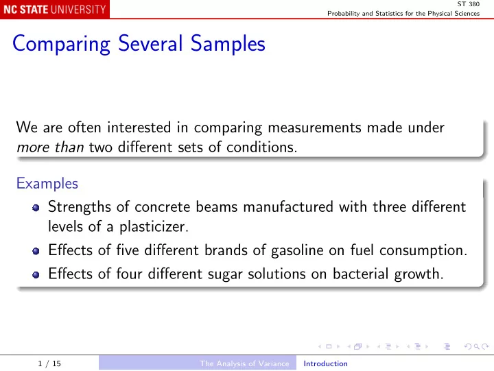
ST 380 Probability and Statistics for the Physical Sciences

Comparing Several Samples

We are often interested in comparing measurements made under more than two different sets of conditions. Examples Strengths of concrete beams manufactured with three different levels of a plasticizer. Effects of five different brands of gasoline on fuel consumption. Effects of four different sugar solutions on bacterial growth.

1 / 15 The Analysis of Variance Introduction

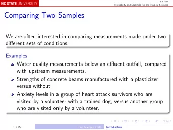
ST 380 Probability and Statistics for the Physical Sciences

Analysis of Variance When we compare more than two samples, we first ask: Are there any differences among populations? If we detect differences, the next question is: Which means are different, and by how much? When there are only two samples, these questions are basically the same; now we have to address them separately. For historical reasons, the techniques are known as the “analysis of variance” (ANOVA).

2 / 15 The Analysis of Variance Analysis of Variance

ST 380 Probability and Statistics for the Physical Sciences

Notation I = the number of samples µ1 = mean of population 1 . . . µI = mean of population I σ2 = the variance in each population Note that the variance is assumed to be the same in each population; no extension of Welch’s method is available.

3 / 15 The Analysis of Variance Analysis of Variance

ST 380 Probability and Statistics for the Physical Sciences

Example 10.1 Four types of boxes were compared in terms of compressive strength (lbf).

boxes <- read.table("Data/Example-10-01.txt", header = TRUE) boxplot(Strength ~ Type, boxes)

Type 4 appears to have lower strength than the other types, and Type 2 appears to be the strongest. How do we make objective statements about these appearances?

4 / 15 The Analysis of Variance Analysis of Variance

ST 380 Probability and Statistics for the Physical Sciences

The first question suggests a hypothesis test: H0 : µ1 = µ2 = · · · = µI versus Ha : at least two of the means are unequal We look for a test statistic that compares the differences among the sample means with what we would expect those differences would be under H0.

5 / 15 The Analysis of Variance Analysis of Variance

ST 380 Probability and Statistics for the Physical Sciences

The conventional statistic is a ratio of sums of squares that are involved in estimating variances, hence “analysis of variance”. Under H0, it follows the F-distribution, and is denoted F. The F-statistic is a generalization of the pooled t-statistic used to compare two samples. ...actually the square of t. The calculations are tedious, and best left to software.

6 / 15 The Analysis of Variance Analysis of Variance

ST 380 Probability and Statistics for the Physical Sciences

Using R

boxesAov <- aov(Strength ~ factor(Type), boxes) summary(boxesAov)

Output

Df Sum Sq Mean Sq F value Pr(>F) factor(Type) 3 127375 42458 25.09 5.53e-07 *** Residuals 20 33839 1692

• Signif. codes:

0 *** 0.001 ** 0.01 * 0.05 . 0.1 1

7 / 15 The Analysis of Variance Analysis of Variance

ST 380 Probability and Statistics for the Physical Sciences

On both the factor(Type) and Residuals lines, the Mean Sq is the Sum Sq divided by the Df. On the factor(Type) line, the F value is the ratio of the mean square for Type to the mean square for Residuals, and is the required test statistic. On the same line, Pr(F) is the P-value, which in this case is less than 10−6; that tells us that there is very strong evidence against H0–no surprise there, given the differences among the box-plots.

8 / 15 The Analysis of Variance Analysis of Variance

ST 380 Probability and Statistics for the Physical Sciences

Multiple Comparisons

When, as in this example, we decide that there are significant differences, the next question is what are they? One approach is to take each pair of samples, and compare them using either: a hypothesis test that the means are equal; a confidence interval for the difference. We have seen that these alternatives are essentially equivalent.

9 / 15 The Analysis of Variance Multiple Comparisons

ST 380 Probability and Statistics for the Physical Sciences

Sometimes this “pairwise” approach is reasonable. However, its error rate may be unacceptable. Among I samples, there are I(I − 1)/2 pairwise comparisons. If we construct I(I − 1)/2 pairwise confidence intervals, each with a probability α of being incorrect, we should expect αI(I − 1)/2 of them to be wrong. If α = .05 and I = 4, as in the example, αI(I − 1)/2 = .3, so the “per-family” error rate is 30%.

10 / 15 The Analysis of Variance Multiple Comparisons

ST 380 Probability and Statistics for the Physical Sciences

Tukey’s HSD Tukey’s “Honest Significant Difference” (HSD) method is a way of constructing pairwise confidence intervals in such a way that the probability that all of them are correct is the desired level (1 − α). Using R

boxesHSD <- TukeyHSD(boxesAov) boxesHSD

11 / 15 The Analysis of Variance Multiple Comparisons

ST 380 Probability and Statistics for the Physical Sciences

Output

Tukey multiple comparisons of means 95% family-wise confidence level Fit: aov(formula = Strength ~ factor(Type), data = boxes) $‘factor(Type)‘ diff lwr upr p adj 2-1 43.93333

• 22.53671

110.403377 0.2804669 3-1

• 14.93333
• 81.40338

51.536711 0.9215560 4-1 -150.98333 -217.45338

• 84.513289 0.0000185

3-2

• 58.86667 -125.33671

7.603377 0.0942542 4-2 -194.91667 -261.38671 -128.446623 0.0000004 4-3 -136.05000 -202.52004

• 69.579956 0.0000726

12 / 15 The Analysis of Variance Multiple Comparisons

ST 380 Probability and Statistics for the Physical Sciences

The results can also be presented graphically:

plot(boxesHSD)

The implications, from both presentantions, are: The confidence intervals for comparing all types except 4 contain zero, so those differences are not significant. The confidence intervals for comparing Type 4 with the other three types are all negative, so Type 4 has significantly lower strength than the other types. Even Though Type 2 appears to be the strongest, that is not confirmed by this experiment.

13 / 15 The Analysis of Variance Multiple Comparisons

ST 380 Probability and Statistics for the Physical Sciences

Inconsistency In some sets of data, the F-test and the HSD may give inconsistent results: The F-test may reject H0, and yet no pair of means are significantly different using the HSD; Conversely, the F-test may fail to reject H0, and yet at least two means are significantly different using the HSD. If your interest really is in pairwise comparisons, for instance to rank the populations, or to find the best or worst, you should ignore the F-test. Just reject H0 if and only if at least two means are significantly different.

14 / 15 The Analysis of Variance Multiple Comparisons

ST 380 Probability and Statistics for the Physical Sciences

False Discovery Rate Other methods than Tukey’s have been proposed for managing the multiplicity problem. When I is large, Tukey’s method may be unnecessarily conservative, meaning that it may fail to detect real differences. Yoav Benjamini and Yosef Hochberg developed the idea of “false discovery rate” as an alternative.

15 / 15 The Analysis of Variance Multiple Comparisons