Comparing Two Samples We are often interested in comparing - PowerPoint PPT Presentation

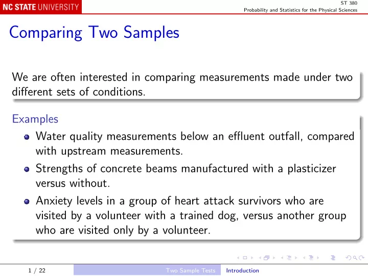
ST 380 Probability and Statistics for the Physical Sciences Comparing Two Samples We are often interested in comparing measurements made under two different sets of conditions. Examples Water quality measurements below an effluent outfall, compared with upstream measurements. Strengths of concrete beams manufactured with a plasticizer versus without. Anxiety levels in a group of heart attack survivors who are visited by a volunteer with a trained dog, versus another group who are visited only by a volunteer. 1 / 22 Two Sample Tests Introduction

ST 380 Probability and Statistics for the Physical Sciences In each case, we have a sample of measurements X 1 , X 2 , . . . , X m made under one set of conditions, and another sample Y 1 , Y 2 , . . . , Y n made under a different set of conditions. Note that the samples are often not of the same size. If the populations have means µ 1 and µ 2 respectively, we usually want to make inferences about the difference µ 1 − µ 2 . We shall want to use the three basic modes of inference: A point estimator of µ 1 − µ 2 . An interval estimator of µ 1 − µ 2 . A test of the null hypothesis H 0 : µ 1 = µ 2 . 2 / 22 Two Sample Tests Comparing Population Means

ST 380 Probability and Statistics for the Physical Sciences Point Estimator Since we have point estimators ¯ X and ¯ Y of µ 1 and µ 2 respectively, the natural point estimator of µ 1 − µ 2 is ¯ X − ¯ Y . Since ¯ X and ¯ Y are unbiased estimators of µ 1 and µ 2 respectively, X − ¯ ¯ Y is an unbiased estimator of µ 1 − µ 2 : E (¯ X − ¯ Y ) = E (¯ X ) − E ( ¯ Y ) = µ 1 − µ 2 . In most cases, we assume that the two samples are independent, and then � σ 2 m + σ 2 � 1 2 σ 2 X + σ 2 σ ¯ Y = Y = X − ¯ ¯ ¯ n 3 / 22 Two Sample Tests Comparing Population Means

ST 380 Probability and Statistics for the Physical Sciences As always, we can estimate σ 2 1 by m 1 � ( X i − ¯ S 2 Y ) 2 1 = m − 1 i =1 and σ 2 2 by n 1 ( Y i − ¯ � S 2 Y ) 2 . 2 = n − 1 i =1 4 / 22 Two Sample Tests Comparing Population Means

ST 380 Probability and Statistics for the Physical Sciences But we often assume that σ 2 1 = σ 2 2 = σ 2 , and estimate the common variance σ 2 by the “pooled” estimate X ) 2 + � n � m i =1 ( X i − ¯ i =1 ( Y i − ¯ Y ) 2 S 2 p = m − 1 + n − 1 = ( m − 1) S 2 1 + ( n − 1) S 2 2 . m + n − 2 We then estimate σ ¯ Y by X − ¯ � � S 2 m + S 2 m + 1 1 p p n = S p n . 5 / 22 Two Sample Tests Comparing Population Means

ST 380 Probability and Statistics for the Physical Sciences Confidence Interval As you might expect, a 100(1 − α )% confidence interval for µ 1 − µ 2 is of the form X − ¯ ¯ Y ± (critical value) α × (standard error) We have three ways of estimating the standard error, and each needs a different critical value. 6 / 22 Two Sample Tests Comparing Population Means

ST 380 Probability and Statistics for the Physical Sciences The simplest case is when the variances are known, or the sample sizes are large enough that they are esssentially known. Then the standard error is � � σ 2 m + σ 2 s 2 m + s 2 1 2 1 2 or n n and the critical value z α/ 2 comes from the normal distribution. 7 / 22 Two Sample Tests Comparing Population Means

ST 380 Probability and Statistics for the Physical Sciences Next, suppose that the variances are unknown but assumed to be equal. Then the standard error is � m + 1 1 s p n and the critical value t α/ 2 , m + n − 2 comes from the t -distribution with ( m + n − 2) degrees of freedom. 8 / 22 Two Sample Tests Comparing Population Means

ST 380 Probability and Statistics for the Physical Sciences The final case, when the variances are unknown and cannot be assumed to be equal, is the most complicated. Then the standard error is � s 2 m + s 2 1 2 n and the critical value t α/ 2 ,ν comes from the t -distribution with ν degrees of freedom, where ν must be calculated from m , n , s 2 1 , and s 2 2 . This is known as Welch’s procedure. 9 / 22 Two Sample Tests Comparing Population Means

ST 380 Probability and Statistics for the Physical Sciences Hypothesis Test When comparing two samples, the null hypothesis is usually H 0 : µ 1 = µ 2 . It could, more generally, be H 0 : µ 1 − µ 2 = δ for some specified δ ; the test is only slightly more complicated. The test is based on X − ¯ ¯ Y T = standard error and the test statistic is either T or | T | , depending on whether the test is one-sided or two-sided. 10 / 22 Two Sample Tests Comparing Population Means

ST 380 Probability and Statistics for the Physical Sciences The calculation of the P -value, or the determination of the critical value for rejection of H 0 , uses: the normal distribution; the t -distribution with ( m + n − 2) degrees of freedom; the t -distribution with Welch’s ν degrees of freedom; depending on the form of the standard error, as in the case of the confidence interval. 11 / 22 Two Sample Tests Comparing Population Means

ST 380 Probability and Statistics for the Physical Sciences Example 9.7: strength of pipe liner Liners used to reinforce a pipeline can be manufactured with or without a certain fusion process. The question is whether the process affects their tensile strength. In R, the t.test() function can be used to test the null hypothesis of equal strength against either two-sided or one-sided alternatives, using either the Welch procedure or the pooled method: liner <- read.table("Data/Example-09-07.txt", header = TRUE) t.test(Strength ~ Fused, liner) t.test(Strength ~ Fused, liner, var.equal = TRUE) t.test() also produces a confidence interval with the same specification as the hypothesis test. 12 / 22 Two Sample Tests Comparing Population Means

ST 380 Probability and Statistics for the Physical Sciences Analysis of Paired Data So far, we have assumed that the two samples were collected in such a way that they are statistically independent. The calculation of the standard error of ¯ X − ¯ Y depended on this assumption. Sometimes the samples are deliberately collected so as not to be independent, to improve the precision of the comparison. 13 / 22 Two Sample Tests Analysis of Paired Data

ST 380 Probability and Statistics for the Physical Sciences Example 9.8: zinc concentration in rivers The question is whether zinc concentrations differ between bottom water ( x ) and surface water ( y ): Data from six locations: Location 1 2 3 4 5 6 0.430 0.266 0.567 0.531 0.707 0.716 x y 0.415 0.238 0.390 0.410 0.605 0.609 x − y 0.015 0.028 0.177 0.121 0.102 0.107 14 / 22 Two Sample Tests Analysis of Paired Data

ST 380 Probability and Statistics for the Physical Sciences Both measurements for a given river are affected by the overall zinc levels in the sources of the river, so we would expect them to be dependent. The scatterplot and the correlation coefficient strongly support dependence: zinc <- read.table("Data/Example-09-08.txt", header = TRUE) with(zinc, plot(Bottom, Surface)) with(zinc, cor(Bottom, Surface)) 15 / 22 Two Sample Tests Analysis of Paired Data

ST 380 Probability and Statistics for the Physical Sciences The conventional analysis of paired data is through the differences: with(zinc, t.test(Bottom - Surface)) t.test() can also work with the two samples, provided you use the paired = TRUE option: with(zinc, t.test(Bottom, Surface, paired = TRUE)) The calculations are the same, but the results are labeled better. 16 / 22 Two Sample Tests Analysis of Paired Data

ST 380 Probability and Statistics for the Physical Sciences The advantage of paired data is that V (¯ X − ¯ Y ) is generally smaller than it would be with independent samples, V (¯ X ) + V ( ¯ Y ): with(zinc, var(Bottom - Surface)) with(zinc, var(Bottom) + var(Surface)) The test has fewer degrees of freedom, which results in lower power, but that is more than compensated by the increase in precision, except when the correlation is very low. 17 / 22 Two Sample Tests Analysis of Paired Data

ST 380 Probability and Statistics for the Physical Sciences Comparing Binomial Parameters Suppose that X ∼ Bin( m , p 1 ) and Y ∼ Bin( n , p 2 ), and that X and Y are independent, and we wish to compare p 1 and p 2 . We have unbiased point estimators p 1 = X p 2 = Y ˆ and ˆ m n of p 1 and p 2 , respectively, so ˆ p 1 − ˆ p 2 is an unbiased estimator of p 1 − p 2 . Also we know the standard error of each, and large-sample normal approximations to their distributions, from which we can derive a confidence interval for p 1 − p 2 . 18 / 22 Two Sample Tests Comparing Population Proportions

ST 380 Probability and Statistics for the Physical Sciences However, it is not clear that “comparing” p 1 and p 2 requires making inferences about the difference p 1 − p 2 . Sometimes the interesting quantity is the log-odds-ratio � p 1 / (1 − p 1 ) � � p 1 � � p 2 � log = log − log p 2 / (1 − p 2 ) 1 − p 1 1 − p 2 So instead of focusing on inference about p 1 − p 2 , we study testing the hypothesis H 0 : p 1 = p 2 = p , because that is the same as equality of the odds ratios. 19 / 22 Two Sample Tests Comparing Population Proportions