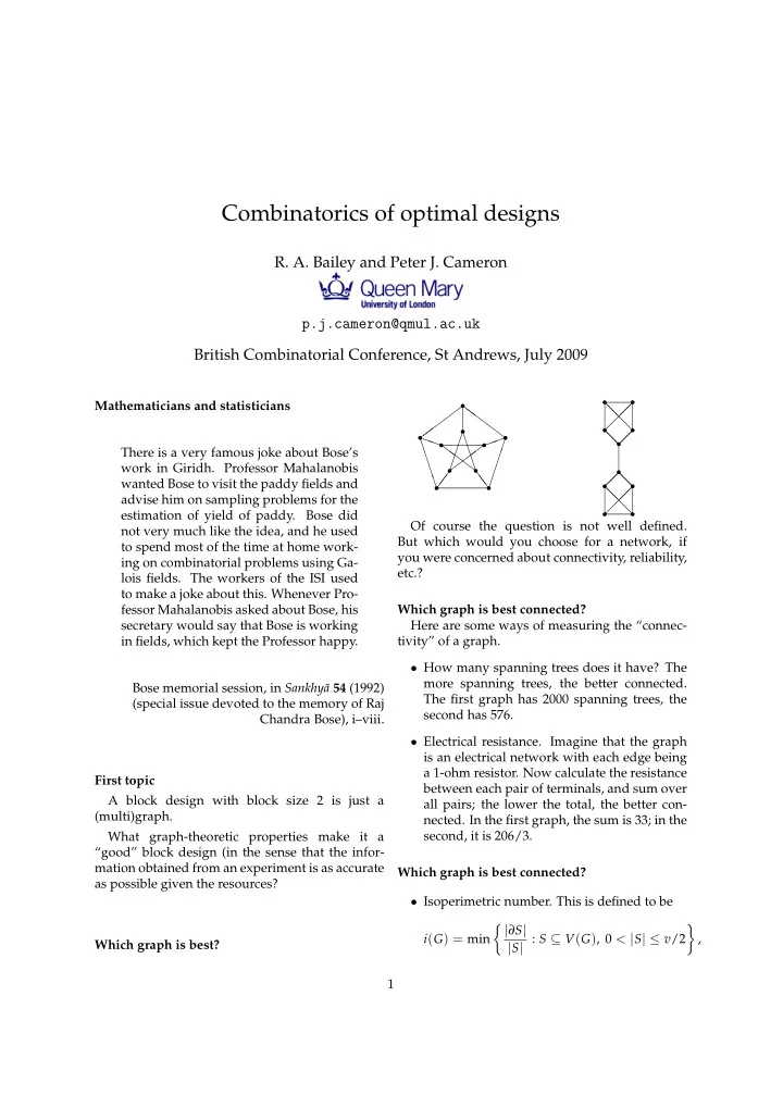

Combinatorics of optimal designs R. A. Bailey and Peter J. Cameron p.j.cameron@qmul.ac.uk British Combinatorial Conference, St Andrews, July 2009 Mathematicians and statisticians r r ✚ ❩ ❅ � r ❩ ❅ � ✚ ❩ � ❅ ✚ ✚ ❩ r r P r ✏ ✂ ❇ ❅ ❅ � � P ✏ r r ❇ ✂ ❩ ✚ r r ✂ ❇ r There is a very famous joke about Bose’s ❩ ✚✚ ✂ ❇ ✂ ❩ ❇ work in Giridh. Professor Mahalanobis ✂ ❇ r r ✓ ❙ r � ❅ � ❅ ❇✓ ❙ ✂ wanted Bose to visit the paddy fields and r r r r ❅ � ❅ � advise him on sampling problems for the � ❅ estimation of yield of paddy. Bose did r r Of course the question is not well defined. not very much like the idea, and he used But which would you choose for a network, if to spend most of the time at home work- you were concerned about connectivity, reliability, ing on combinatorial problems using Ga- etc.? lois fields. The workers of the ISI used to make a joke about this. Whenever Pro- fessor Mahalanobis asked about Bose, his Which graph is best connected? secretary would say that Bose is working Here are some ways of measuring the “connec- in fields, which kept the Professor happy. tivity” of a graph. • How many spanning trees does it have? The more spanning trees, the better connected. Bose memorial session, in Sankhy¯ a 54 (1992) The first graph has 2000 spanning trees, the (special issue devoted to the memory of Raj second has 576. Chandra Bose), i–viii. • Electrical resistance. Imagine that the graph is an electrical network with each edge being a 1-ohm resistor. Now calculate the resistance First topic between each pair of terminals, and sum over A block design with block size 2 is just a all pairs; the lower the total, the better con- (multi)graph. nected. In the first graph, the sum is 33; in the What graph-theoretic properties make it a second, it is 206/3. “good” block design (in the sense that the infor- mation obtained from an experiment is as accurate Which graph is best connected? as possible given the resources? • Isoperimetric number. This is defined to be � | ∂ S | � i ( G ) = min | S | : S ⊆ V ( G ) , 0 < | S | ≤ v /2 , Which graph is best? 1
There is also an upper bound for i ( G ) in terms where, for a set S of vertices, ∂ S is the set of edges from S to its complement. Large of µ 1 , an inequality of Cheeger type , which is crucial isoperimetric number means that there are for other applications (to random walks etc.) many edges out of any set of vertices. The Recently, Krivelevich and Sudakov have shown isoperimetric number for the first graph is that, in a k -regular graph G on v vertices, if µ 1 is 1 (there are just five edges between the in- large enough in terms of v and k , then G is Hamil- ner and outer pentagons), that of the second tonian. Pyber used this to show that all but finitely graph is 1/5 (there is just one edge between many strongly regular graphs are Hamiltonian. the top and bottom components). Graphs as block designs Laplacian eigenvalues Suppose that we have ten “treatments” that we Let G be a graph on n vertices. (Multiple edges want to compare. We have enough resources to are allowed but loops are not.) perform fifteen trials, each one of which compares The Laplacian matrix of G is the n × n matrix two of the treatments. L ( G ) whose ( i , i ) entry is the number of edges con- The trials can be regarded as the edges of a taining vertex i , while for i � = j the ( i , j ) entry is the graph with 10 vertices and 15 edges. So our negative of the number of edges joining vertices i two examples are among the graphs we could and j . use. Which will give the best possible information This is a real symmetric matrix; its eigenvalues about treatment differences? are the Laplacian eigenvalues of G . Note that its row We model the result of each trial as giving a sums are zero. number for each of the two treatments in the trial, which is the sum of an effect due to a treatment, an effect due to the trial, and some random variation. Laplacian eigenvalues • L ( G ) is positive semi-definite, so its eigenval- Treatment contrasts ues are non-negative. We cannot estimate treatment effects directly, because adding the same quantity to each treat- • The multiplicity of 0 as an eigenvalue of G ment effect and subtracting it from each trial effect is equal to the number of connected compo- will not change the results. nents of G . In particular, if G is connected, We can estimate treatment differences , or more then 0 is a simple eigenvalue (called the triv- generally treatment contrasts , linear combinations ial eigenvalue ) corresponding to the all-1 eigen- of treatment effects where the coefficients sum to vector, and the non-trivial eigenvalues are zero. positive. Each treatment contrast estimator is a random variable, and the smaller its variance, the more ac- • The number of spanning trees of G is the curate the estimate. Accurate estimates are impor- product of the non-trivial Laplacian eigenval- tant to reduce the risk that we rate one treatment ues, divided by v : this is Kirchhoff’s Matrix- better than another just because of random varia- Tree Theorem . tion. Laplacian eigenvalues Optimality criteria • The sum of resistances between all pairs of Among desirable criteria we might ask for an vertices is the sum of reciprocals of the non- experimental design to do one of the following: trivial Laplacian eigenvalues, multiplied by v . • minimize the average variance of the treat- • The isoperimetric number is at least half of the ment differences (such a design is called A- smallest non-trivial eigenvalue of G . optimal ); 2
• minimize the volume of a confidence ellipsoid Mathematicians tend to represent a block de- containing the estimated treatment contrasts sign by a family of subsets of the treatment set, (such a design is called D-optimal ; where each block corresponds to a set of k treat- ments. There are different schools of thought • minimize the maximum variance of any nor- about whether “repeated blocks” should be al- malised treatment contrast (such a design is lowed. called E-optimal ). In fact there is a much more serious problem . . . There are other types of optimality too, but these will do for now! (For D-optimality, we need to as- An example sume the errors are independent normal.) We have five treatments numbered 1, . . . , 5, and 21 experimental units, divided into seven blocks Optimality and graph properties of three. The design is given in the following table: Theorem 1. In any given class of graphs, 1 1 1 1 2 2 2 • the A-optimal graph mimimizes the sum of resis- 1 3 3 4 3 3 4 tances between all pairs of vertices; 2 4 5 5 4 5 5 • the D-optimal graph maximizes the number of spanning trees in the graph; A combinatorialist wanting to represent this block design in the “traditional” way, with blocks • the E-optimal graph maximizes the minimum non- as subsets of the set of treatments, has a problem: trivial Laplacian eigenvalue of the graph. the first block is a multiset [ 1, 1, 2 ] . Nevertheless, to a statistician there is no prob- So E-optimal graphs will tend to have large lem with this; indeed, it can be shown that this isoperimetric numbers. design is E-optimal among all designs for 5 treat- ments and 7 blocks of size 3. Second topic A block design with block size greater than 2 is not a graph. Perhaps we should regard it as a hy- An example, continued pergraph of some kind? Look at the example again: It will turn out that optimality properties of such a block design are determined by a graph, the con- 1 1 1 1 2 2 2 currence graph of the block design, no matter what 1 3 3 4 3 3 4 the block size. So we do not need a new theory! 2 4 5 5 4 5 5 1 and 2 occur together twice in the first block. What is a block design? With this convention, you can easily check that We wish to do an experiment to test v differ- the block design is balanced , that is, the equivalent ent treatments. We have available bk experimen- of a 2-design: every pair of treatments lie together tal units, divided into b “blocks” of k ; there are in exactly two blocks. systematic but unknown differences between the We have called these designs “variance- blocks. We model the response of an experimental balanced designs” or VB-designs in the paper; unit as the sum of a treatment effect, a block effect, some statisticians call them “completely sym- and random variation, and we want to estimate metric designs” (a term unlikely to appeal to treatment differences, or more generally, treatment mathematicians)! contrasts. For example, we may be testing varieties of It is known that VB-designs are E-optimal as seed, and have k plots available for planting the long as they don’t have too much “badness” (mul- seed on each of b farms in different geographic and tiple occurrences of treatments in blocks). See the climatic areas. paper for details. 3
Recommend
More recommend