Clustering Lecture notes Clustering is Exploratory, unsupervised - PowerPoint PPT Presentation

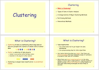
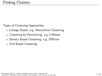
Clustering Lecture notes

Clustering is Exploratory, unsupervised method Data in cluster is similar to each other, and dissimilar to other cluster data Finding structure in data Hard vs. Soft/Fuzzy vs. Exclusive Understanding and/or summarise 70% 15% Hard vs Fuzzy/Soft clustering 13% 2%

Types of clusters Well separated Overlapping Contiguity Centre-based – based on distance to cluster centres. points are closer to others in their cluster than any other cluster Conceptual Density Sharing some general High-density areas attribute. Intersections separated by low-density belong to both areas

Notion of cluster ambiguous

Applications Biology – compare species in different environments Medicine – Group variants of illnesses or similar genes PET scans; differentiate tissues Marketing – Consumers with similar shopping habits, grouping shopping items Social sciences – Crime analysis (greatest incidences of different crimes), Poll data Computer science – Data compression, Anomaly detection Internet – Web searches (categories of results), social media analysis Other : Location of network towers for optimum signal cover Netflix (cluster similar view habits) Group skulls from archeological digs based on measurements

“Distance” metric • Minkowski metric Others metrics • Mahalanobis distance – Absolute without redundancies for n features, points x,y • Pearson correlation (unit indep.) – covariance(x,y) / [std(x) std(y)] Bad for high dimension data • Binary data: – Russel, Dice, Yule index, …. Two common cases: Manhattan, q = 1 • Cosine (Document: keywords) (cityblock) • Gowder’s distance (mixed) Euclidean, q = 2 • Alternatives (squared distances): (“as the crow flies”) ✴ Squared Euclidean Magnitude and units affect ✴ Squared Pearson (e.g. body height vs. toe length) ………. -> standardise ! (mean=0, std=1) But may affect variability

Linkage criteria Represent cluster location nearest(single) neighbour (noise,outliers) farthest(complete) neighbour (noise,outliers,favours global shape) average – calculate avg. amongst point dist. (middle of single/complete) centroid – virtual "average" point based on each feature medoid – real “median" point

Example calculation 4 B 3 2 A 1 1 2 3 4 5 6

Distance comparison Manhattan Euclidean Single 4 sqrt(8)=2.83 Complete 7 sqrt(29)=5.39 Average 48/9=5.33 4.00 Centroid 16/3 = 5.33 sqrt(153/9)=4.12 Medoid 6 sqrt(18)=4.24

Hierarchical (Hierarchical) tree of nested clusters Levels are steps in clustering process agglomerative vs divisive “bottom-up” vs “top-down” Time complexity at least n^2 Divisive often more computationally demanding

Dendrogram a 9 8 b 7 c 6 5 d 4 3 2 e Stepwise merge or split 1 1 2 3 4 5 6 7 8 9

Dendrogram Root Branch Root – starting point for point all points Branch point – Threshold splitting/merging point Leaf – point is in its own cluster Threshold – selected limit for best # clusters Leaf

Example calculation – Revisited 5 a b c 4 a b c d e a 0 1 4 5 5 3 b 1 0 2 6 6 d 2 c 4 2 0 7 7 e d 5 6 7 0 2 1 e 5 6 7 2 0 1 2 3 4 5 6 Manhattan metric with centroid linkage

Example calculation – Revisited ab 5 c 4 ab c d e 3 ab 0 3.5 5.5 5.5 d c 3.5 0 7 7 2 d 5.5 7 0 2 e 1 e 5.5 7 2 0 1 2 3 4 5 6 Manhattan metric with centroid linkage

Example calculation – Revisited ab 5 c 4 ab c de 3 ab 0 4.5 5 2 c 4.5 0 7 de 1 de 5 7 0 1 2 3 4 5 6 Manhattan metric with centroid linkage

Example calculation – Revisited 5 abc c 4 3 2 de 1 1 2 3 4 5 6 Manhattan metric with centroid linkage

More detailed example

k-means Partitional clustering method Specify number of clusters k , find the most compact solution Ordinarily time complexity n dk+1 for d=features, k=clusters Faster algorithms exist (Lloyd's algorithm is linear!) But, k-means falls into local minima , several trials needed and only handles numeric data and redundancies are not excluded

k-means – Initialise Initialise k cluster centroids randomly – possibly different clusters, do multiple runs first random or average, then rest most distant point for centroids – may select outliers) k means++ (first is fully random, the others random with probability proportional to D 2 – distance to nearest centroid) then …….

k-means – Iterate Iterate (determine:) calculate centroids calculate distances to centroids move points to closest centroid Repeat until either: No points move clusters <X% moves Maximum iterations

k-means – issues Empty clusters – replace centroid with farthest point to clusters or from cluster with highest Sum of Square Errors Outliers – Points with high contribution to cluster SSE, and more But for some fields, like financial, outliers are important

Visualisation – k= 10, white crosses are centroids

Silhouette What k to use? Validates performance based on intra and inter-cluster distances a(i) average dissimilarity with other data in cluster b(i) lowest dissimilarity to any non-member cluster Values [-1,1] Calculated for each point, so very time demanding!

Calinski-Harabasz Index Faster , better for large data Performance based on average intra and inter-cluster SSE (Tr):

Postprocessing We may still want to improve SSE of our results • Split cluster with largest SSE or standard deviation • Open a new cluster using point most distant to any cluster Decrease number of clusters with smallest SSE increase • Disperse a cluster, reassign points to cluster increasing SSE the least • Merge two clusters with the closest centroids