Non-Bayesian Classifiers Part I: k -Nearest Neighbor Classifier and - PowerPoint PPT Presentation
Non-Bayesian Classifiers Part I: k -Nearest Neighbor Classifier and Distance Functions Selim Aksoy Department of Computer Engineering Bilkent University saksoy@cs.bilkent.edu.tr CS 551, Spring 2019 CS 551, Spring 2019 2019, Selim Aksoy
Non-Bayesian Classifiers Part I: k -Nearest Neighbor Classifier and Distance Functions Selim Aksoy Department of Computer Engineering Bilkent University saksoy@cs.bilkent.edu.tr CS 551, Spring 2019 CS 551, Spring 2019 � 2019, Selim Aksoy (Bilkent University) c 1 / 13
Non-Bayesian Classifiers ◮ We have been using Bayesian classifiers that make decisions according to the posterior probabilities. ◮ We have discussed parametric and non-parametric methods for learning classifiers by estimating the probabilities using training data. ◮ We will study new techniques that use training data to learn the classifiers directly without estimating any probabilistic structure. ◮ In particular, we will study the k -nearest neighbor classifier, linear discriminant functions, and support vector machines. CS 551, Spring 2019 � 2019, Selim Aksoy (Bilkent University) c 2 / 13
The Nearest Neighbor Classifier ◮ Given the training data D = { x 1 , . . . , x n } as a set of n labeled examples, the nearest neighbor classifier assigns a test point x the label associated with its closest neighbor in D . ◮ Closeness is defined using a distance function. ◮ Given the distance function, the nearest neighbor classifier partitions the feature space into cells consisting of all points closer to a given training point than to any other training points. CS 551, Spring 2019 � 2019, Selim Aksoy (Bilkent University) c 3 / 13
The Nearest Neighbor Classifier ◮ All points in such a cell are labeled by the class of the training point, forming a Voronoi tesselation of the feature space. Figure 1: In two dimensions, the nearest neighbor algorithm leads to a partitioning of the input space into Voronoi cells, each labeled by the class of the training point it contains. In three dimensions, the cells are three-dimensional, and the decision boundary resembles the surface of a crystal. CS 551, Spring 2019 � 2019, Selim Aksoy (Bilkent University) c 4 / 13
The k -Nearest Neighbor Classifier ◮ The k -nearest neighbor classifier classifies x by assigning it the label most frequently represented among the k nearest samples. ◮ In other words, a decision is made by examining the labels on the k -nearest neighbors and taking a vote. Figure 2: The k -nearest neighbor query forms a spherical region around the test point x until it encloses k training samples, and it labels the test point by a majority vote of these samples. In the case for k = 5 , the test point will be labeled as black. CS 551, Spring 2019 � 2019, Selim Aksoy (Bilkent University) c 5 / 13
The k -Nearest Neighbor Classifier ◮ The computational complexity of the nearest neighbor algorithm — both in space (storage) and time (search) — has received a great deal of analysis. ◮ In the most straightforward approach, we inspect each stored training point one by one, calculate its distance to x , and keep a list of the k closest ones. ◮ There are some parallel implementations and algorithmic techniques for reducing the computational load in nearest neighbor searches. CS 551, Spring 2019 � 2019, Selim Aksoy (Bilkent University) c 6 / 13
The k -Nearest Neighbor Classifier ◮ Examples of algorithmic techniques include ◮ computing partial distances using a subset of dimensions, and eliminating the points with partial distances greater than the full distance of the current closest points, ◮ using search trees that are hierarchically structured so that only a subset of the training points are considered during search, ◮ editing the training set by eliminating the points that are surrounded by other training points with the same class label. CS 551, Spring 2019 � 2019, Selim Aksoy (Bilkent University) c 7 / 13
Distance Functions ◮ The nearest neighbor classifier relies on a metric or a distance function between points. ◮ For all points x , y and z , a metric D ( · , · ) must satisfy the following properties: ◮ Nonnegativity: D ( x , y ) ≥ 0 . ◮ Reflexivity: D ( x , y ) = 0 if and only if x = y . ◮ Symmetry: D ( x , y ) = D ( y , x ) . ◮ Triangle inequality: D ( x , y ) + D ( y , z ) ≥ D ( x , z ) . ◮ If the second property is not satisfied, D ( · , · ) is called a pseudometric. CS 551, Spring 2019 � 2019, Selim Aksoy (Bilkent University) c 8 / 13
Distance Functions ◮ A general class of metrics for d -dimensional patterns is the Minkowski metric � d � 1 /p � | x i − y i | p L p ( x , y ) = i =1 also referred to as the L p norm . ◮ The Euclidean distance is the L 2 norm � d � 1 / 2 � | x i − y i | 2 L 2 ( x , y ) = . i =1 ◮ The Manhattan or city block distance is the L 1 norm d � L 1 ( x , y ) = | x i − y i | . i =1 CS 551, Spring 2019 � 2019, Selim Aksoy (Bilkent University) c 9 / 13
Distance Functions ◮ The L ∞ norm is the maximum of the distances along individual coordinate axes d L ∞ ( x , y ) = max i =1 | x i − y i | . Figure 3: Each colored shape consists of points at a distance 1.0 from the origin, measured using different values of p in the Minkowski L p metric. CS 551, Spring 2019 � 2019, Selim Aksoy (Bilkent University) c 10 / 13
Feature Normalization ◮ We should be careful about scaling of the coordinate axes when we compute these metrics. ◮ When there is great difference in the range of the data along different axes in a multidimensional space, these metrics implicitly assign more weighting to features with large ranges than those with small ranges. ◮ Feature normalization can be used to approximately equalize ranges of the features and make them have approximately the same effect in the distance computation. ◮ The following methods can be used to independently normalize each feature. CS 551, Spring 2019 � 2019, Selim Aksoy (Bilkent University) c 11 / 13
Feature Normalization ◮ Linear scaling to unit range: Given a lower bound l and an upper bound u for a feature x ∈ R , x = x − l ˜ u − l results in ˜ x being in the [0 , 1] range. ◮ Linear scaling to unit variance: A feature x ∈ R can be transformed to a random variable with zero mean and unit variance as x = x − µ ˜ σ where µ and σ are the sample mean and the sample standard deviation of that feature, respectively. CS 551, Spring 2019 � 2019, Selim Aksoy (Bilkent University) c 12 / 13
Feature Normalization ◮ Normalization using the cumulative distribution function: Given a random variable x ∈ R with cumulative distribution function F x ( x ) , the random variable ˜ x resulting from the transformation ˜ x = F x ( x ) will be uniformly distributed in [0 , 1] . ◮ Rank normalization: Given the sample for a feature as x 1 , . . . , x n ∈ R , first we find the order statistics x (1) , . . . , x ( n ) and then replace each pattern’s feature value by its corresponding normalized rank as x 1 ,...,x n ( x i ) − 1 rank ˜ x i = n − 1 where x i is the feature value for the i ’th pattern. This procedure uniformly maps all feature values to the [0 , 1] range. CS 551, Spring 2019 � 2019, Selim Aksoy (Bilkent University) c 13 / 13
Recommend
More recommend
Explore More Topics
Stay informed with curated content and fresh updates.
