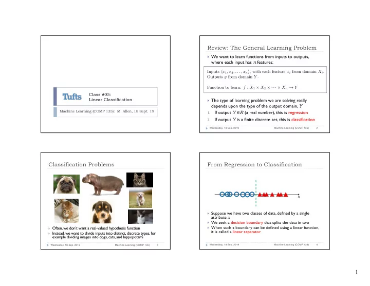
Classification Problems From Regression to Classification x } - PowerPoint PPT Presentation

Review: The General Learning Problem } We want to learn functions from inputs to outputs, where each input has n features: Inputs h x 1 , x 2 , . . . , x n i , with each feature x i from domain X i . Outputs y from domain Y . Function to learn: f : X 1 ⇥ X 2 ⇥ · · · ⇥ X n ! Y Class #05: Linear Classification } The type of learning problem we are solving really depends upon the type of the output domain, Y Machine Learning (COMP 135): M. Allen, 18 Sept. 19 If output Y ∈ R (a real number) , this is regression 1. If output Y is a finite discrete set, this is classification 2. 2 Wednesday, 18 Sep. 2019 Machine Learning (COMP 135) Classification Problems From Regression to Classification x } Suppose we have two classes of data, defined by a single attribute x } We seek a decision boundary that splits the data in two } When such a boundary can be defined using a linear function, } Often, we don’t want a real-valued hypothesis function it is called a linear separator } Instead, we want to divide inputs into distinct, discrete types, for example dividing images into dogs, cats, and hippopotami 4 Wednesday, 18 Sep. 2019 Machine Learning (COMP 135) 3 Wednesday, 18 Sep. 2019 Machine Learning (COMP 135) 1

Threshold Functions From Regression to Classification We have data-points with n features: 1. x = ( x 1 , x 2 , . . . , x n ) We have a linear function defined by n +1 weights: 2. w = ( w 0 , w 1 , w 2 , . . . , w n ) x We can write this linear function as: 3. w · x We can then find the linear boundary, where: 4. } Data is linearly separable if it can be divided into classes using w · x = 0 a linear boundary: And use it to define our threshold between classes: 5. w · x = 0 ( Outputs 1 and 0 here are 1 w · x ≥ 0 } Such a boundary, in 1 -dimensional space, is a threshold value h w = arbitrary labels for one 0 w · x < 0 of two possible classes 6 Wednesday, 18 Sep. 2019 Machine Learning (COMP 135) 5 Wednesday, 18 Sep. 2019 Machine Learning (COMP 135) From Regression to Classification From Regression to Classification Image: R. Urtasun (U. of Toronto) } Data is linearly separable if it can be divided into classes } Data is linearly separable if it can be divided into classes using a using a linear boundary: linear boundary: w · x = 0 w · x = 0 } Such a boundary, in 2 -dimensional space, is a line } Such a boundary, in 3 -dimensional space, is a plane } In higher dimensions, it is a hyper-plane 8 Wednesday, 18 Sep. 2019 Machine Learning (COMP 135) 7 Wednesday, 18 Sep. 2019 Machine Learning (COMP 135) 2

The Geometry of Linear Boundaries The Geometry of Linear Boundaries x 2 x 2 } For example, with “real” weights: } Suppose we have 2 - dimensional inputs w = ( w 1 , w 2 ) = (0 . 5 , 1 . 0) x = ( x 1 , x 2 ) 2.0 we get the vector shown } The “real” weights as a green arrow w · x = w 0 + w · ( x 1 , x 2 ) = 0 w = ( w 1 , w 2 ) 1.5 } Then, for a bias weight define a vector w 0 = − 1 . 0 − w 0 /w 2 } The boundary where our 1.0 the boundary where our linear function is zero, w · x = w 0 + w · ( x 1 , x 2 ) = 0 linear function is zero, w w · x = w 0 + w · ( x 1 , x 2 ) = 0 0.5 w · x = w 0 + w · ( x 1 , x 2 ) = 0 is an orthogonal line, is the line shown in red, x 1 x 1 parallel to w · ( x 1 , x 2 ) = 0 0.0 crossing origin at (2,0) & (0,1) − w 0 /w 1 } Its offset from origin is 0.0 0.5 1.0 1.5 2.0 determined by w 0 (which is w · ( x 1 , x 2 ) = 0 called the bias weight) 10 Wednesday, 18 Sep. 2019 Machine Learning (COMP 135) 9 Wednesday, 18 Sep. 2019 Machine Learning (COMP 135) The Geometry of Linear Boundaries Zero-One Loss x 2 x 2 } For a training set made up of } Once we have our linear input/output pairs, boundary, data points are { ( x 1 , y 1 ) , ( x 2 , y 2 ) , . . . , ( x k , y k ) } classified according to our we could define the threshold function zero/one loss h w = 1 ( 1 w · x ≥ 0 ( 0 if h w ( x i ) = y i h w = ( w · x ≥ 0) L ( h w ( x i ) , y i ) = 0 w · x < 0 1 if h w ( x i ) 6 = y i } Summed for the entire set, h w = 0 this is simply the count of ( w · x < 0) examples that we get wrong x 1 x 1 w · x = 0 } In this example, if data-points marked should be in class 0 (below the line) and those marked should be in class 1 (above the line) the loss would be equal to 3 12 Wednesday, 18 Sep. 2019 Machine Learning (COMP 135) 11 Wednesday, 18 Sep. 2019 Machine Learning (COMP 135) 3

Minimizing Zero/One Loss Perceptron Loss } Sadly, it is not easy to compute weights that minimize zero/one loss } Instead, we define the perceptron loss on a training item: } It is a piece-wise constant function of weights x i = ( x i, 1 , x i, 2 , . . . , x i,n ) } It is not continuous, however, and gradient descent won’t work n X L π ( h w ( x i ) , y i ) = ( y i − h w ( x i )) × x i,j } E.g., for the following one-dimensional data, we get loss shown below: j =0 x 1 } For example, suppose we have a 2 -dimensional element in our 0 1 2 3 4 5 6 7 training set for which the correct output is 0 , but our Loss threshold function says 1 : 2 x i = (0 . 5 , 0 . 4) y i = 1 h w ( x i ) = 0 L π ( h w ( x i ) , y i ) = (1 − 0)(1 + 0 . 5 + 0 . 4) = 1 . 9 1 Sum of input attributes ( 1 is the “dummy” The difference between what output x 1 0 should be, and what our weights make it attribute that is multiplied by bias weight w 0 ) 0 1 2 3 4 5 6 7 14 Wednesday, 18 Sep. 2019 Machine Learning (COMP 135) 13 Wednesday, 18 Sep. 2019 Machine Learning (COMP 135) Perceptron Learning Perceptron Updates } T o minimize perceptron loss we can start from initial weights— w j ← w j + α ( y − h w ( x i )) × x i,j perhaps chosen uniformly from interval [-1,1] —and then: } The perceptron update rule shifts the weight vector positively or negatively, Choose an input x i from our data set that is wrongly classified. 1. trying to get all data on the right side of the linear decision boundary Update vector of weights, , as follows: w = ( w 0 , w 1 , w 2 , . . . , w n ) 2. } Again, supposing we have an error as before, with weights as given below: w j ← w j + α ( y i − h w ( x i )) × x i,j x i = (0 . 5 , 0 . 4) w = (0 . 2 , − 2 . 5 , 0 . 6) y i = 1 Repeat until no classification errors remain. 3. w · x i = 0 . 2 + ( − 2 . 5 × 0 . 5) + (0 . 6 × 0 . 4) = − 0 . 81 h w ( x i ) = 0 } The update equation means that: } This means we add the value of each attribute to its matching weight If correct output should be below the boundary ( y i = 0 ) but our 1. (assuming again that “dummy” x i,0 = 1 , and that parameter 𝛽 = 1 ): threshold has placed it above ( h w ( x i ) = 1 ) then we subtract each After adjusting weights, feature ( x i,j ) from the corresponding weight ( w i ) w 0 ← ( w 0 + x i, 0 ) = (0 . 2 + 1) = 1 . 2 our function is now If correct output should be above the boundary ( y i = 1 ) but our w 1 ← ( w 1 + x i, 1 ) = ( − 2 . 5 + 0 . 5) = − 2 . 0 2. correct on this input threshold has placed it below ( h w ( x i ) = 0 ) then we add each w 2 ← ( w 2 + x i, 2 ) = (0 . 6 + 0 . 4) = 1 . 0 feature ( x i,j ) to the corresponding weight ( w i ) w · x i = 1 . 2 + ( − 2 . 0 × 0 . 5) + (1 . 0 × 0 . 4) = 0 . 6 h w ( x i ) = 1 16 Wednesday, 18 Sep. 2019 Machine Learning (COMP 135) 15 Wednesday, 18 Sep. 2019 Machine Learning (COMP 135) 4

Progress of Perceptron Learning Progress of Perceptron Learning x 2 x 2 } For an example like this, we: } Once we get a new boundary, we repeat the process Choose a mis-classified item 1. Choose a mis-classified item (marked in green) 1. (marked in green) Compute the weight updates, 2. Compute the weight updates, 2. based on the “distance” away based on the “distance” away from the boundary (so weights from the boundary (so weights shift more based upon errors in shift more based upon errors in boundary placement that are boundary placement that are more extreme) more extreme) } Here, this subtracts from each } Here, this adds to each weight, weight, changing the decision x 1 x 1 changing the decision boundary boundary in the other direction } In this example, data-points marked should be in class 0 (below } In this example, data-points marked should be in class 0 (below the line) and those marked should be in class 1 (above the line) the line) and those marked should be in class 1 (above the line) 18 Wednesday, 18 Sep. 2019 Machine Learning (COMP 135) 17 Wednesday, 18 Sep. 2019 Machine Learning (COMP 135) Linear Separability Linearly Inseparable Data x 2 x 2 } The process of adjusting } Some data can’t be separated weights stops when there is using a linear classifier no classification error left } Any line drawn will always leave } A data-set is linearly separable some error if a linear separator exists for } The perceptron update which there will be no error method is guaranteed to eventually converge to an } It is possible that there are error-free boundary if such a multiple linear boundaries boundary really exists that achieve this } If it doesn’t exist, then the most } It is also possible that there is x 1 x 1 basic version of the algorithm no such boundary! will never terminate 20 Wednesday, 18 Sep. 2019 Machine Learning (COMP 135) 19 Wednesday, 18 Sep. 2019 Machine Learning (COMP 135) 5