Classification Algorithms UCSB 293S, 2017. T. Yang Some of slides - PowerPoint PPT Presentation
Classification Algorithms UCSB 293S, 2017. T. Yang Some of slides based on R. Mooney (UT Austin) 1 Table of Content Problem Definition Rocchio K-nearest neighbor (case based) Bayesian algorithm Decision trees SVM 2
Classification Algorithms UCSB 293S, 2017. T. Yang Some of slides based on R. Mooney (UT Austin) 1
Table of Content • Problem Definition • Rocchio • K-nearest neighbor (case based) • Bayesian algorithm • Decision trees • SVM 2
Classification • Given: – A description of an instance, x – A fixed set of categories (classes): C= { c 1 , c 2 ,… c n } – Training examples • Determine: – The category of x : h ( x ) Î C, where h ( x ) is a classification function • A training example is an instance x, paired with its correct category c ( x ): < x , c ( x )> 3
Sample Learning Problem • Instance space: <size, color, shape> – size Î {small, medium, large} – color Î {red, blue, green} – shape Î {square, circle, triangle} • C = {positive, negative} • D : Example Size Color Shape Category 1 small red circle positive 2 large red circle positive 3 small red triangle negative 4 large blue circle negative 4
General Learning Issues • Many hypotheses are usually consistent with the training data. • Bias – Any criteria other than consistency with the training data that is used to select a hypothesis. • Classification accuracy (% of instances classified correctly). – Measured on independent test data. • Training time (efficiency of training algorithm). • Testing time (efficiency of subsequent classification). 5
Text Categorization/Classification • Assigning documents to a fixed set of categories. • Applications: – Web pages • Recommending/ranking • category classification – Newsgroup Messages • Recommending • spam filtering – News articles • Personalized newspaper – Email messages • Routing • Prioritizing • Folderizing • spam filtering 6
Learning for Classification • Manual development of text classification functions is difficult. • Learning Algorithms: – Bayesian (naïve) – Neural network – Rocchio – Rule based (Ripper) – Nearest Neighbor (case based) – Support Vector Machines (SVM) – Decision trees – Boosting algorithms 7
Illustration of Rocchio method 8
Rocchio Algorithm Assume the set of categories is { c 1 , c 2 ,… c n } Training: Each doc vector is the frequency normalized TF/IDF term vector. For i from 1 to n Sum all the document vectors in c i to get prototype vector p i Testing: Given document x Compute the cosine similarity of x with each prototype vector. Select one with the highest similarity value and return its category 9
Rocchio Anomoly • Prototype models have problems with polymorphic (disjunctive) categories. 10
Nearest-Neighbor Learning Algorithm • Learning is just storing the representations of the training examples in D . • Testing instance x : – Compute similarity between x and all examples in D . – Assign x the category of the most similar example in D . • Does not explicitly compute a generalization or category prototypes. • Also called: – Case-based – Memory-based – Lazy learning 11
K Nearest-Neighbor • Using only the closest example to determine categorization is subject to errors due to: – A single atypical example. – Noise (i.e. error) in the category label of a single training example. • More robust alternative is to find the k most-similar examples and return the majority category of these k examples. • Value of k is typically odd to avoid ties, 3 and 5 are most common. 12
Similarity Metrics • Nearest neighbor method depends on a similarity (or distance) metric. • Simplest for continuous m -dimensional instance space is Euclidian distance . • Simplest for m -dimensional binary instance space is Hamming distance (number of feature values that differ). • For text, cosine similarity of TF-IDF weighted vectors is typically most effective. 13
3 Nearest Neighbor Illustration (Euclidian Distance) . . . . . . . . . . . 14
K Nearest Neighbor for Text Training: For each each training example < x , c ( x )> Î D Compute the corresponding TF-IDF vector, d x , for document x Test instance y : Compute TF-IDF vector d for document y For each < x , c ( x )> Î D Let s x = cosSim( d , d x ) Sort examples, x , in D by decreasing value of s x Let N be the first k examples in D. ( get most similar neighbors ) Return the majority class of examples in N 15
Illustration of 3 Nearest Neighbor for Text 16
Bayesian Classification 17
Bayesian Methods • Learning and classification methods based on probability theory. – Bayes theorem plays a critical role in probabilistic learning and classification. • Uses prior probability of each category – Based on training data • Categorization produces a posterior probability distribution over the possible categories given a description of an item. 18
Basic Probability Theory • All probabilities between 0 and 1 £ £ 0 P ( A ) 1 • True proposition has probability 1, false has probability 0. P(true) = 1 P(false) = 0. • The probability of disjunction is: Ú = + - Ù P ( A B ) P ( A ) P ( B ) P ( A B ) A Ù B A B 19
Conditional Probability • P( A | B ) is the probability of A given B • Assumes that B is all and only information known. • Defined by: Ù P ( A B ) = P ( A | B ) P ( B ) A Ù B A B 20
Independence • A and B are independent iff: = P ( A | B ) P ( A ) These two constraints are logically equivalent = P ( B | A ) P ( B ) • Therefore, if A and B are independent: Ù P ( A B ) = = P ( A | B ) P ( A ) P ( B ) Ù = P ( A B ) P ( A ) P ( B ) 21
Joint Distribution • Joint probability distribution for X 1 ,…, X n gives the probability of every combination of values: P( X 1 ,…, X n ) – All values must sum to 1. negative Category=positive Color\shape circle square circle square red 0.05 0.30 red 0.20 0.02 blue 0.20 0.20 blue 0.02 0.01 • Probability for assignments of values to some subset of variables can be calculated by summing the appropriate subset Ù circle = + = P ( red ) 0 . 20 0 . 05 0 . 25 = + + + = P ( red ) 0 . 20 0 . 02 0 . 05 0 . 3 0 . 57 • Conditional probabilities can also be calculated. Ù Ù P ( positive red circle ) 0 . 20 Ù = = = P ( positive | red circle ) 0 . 80 Ù P ( red circle ) 0 . 25 22
Computing probability from a training dataset Probability Y=positive negative Ex Size Color Shape Category P( Y ) 0.5 0.5 1 small red circle positive P(small | Y ) 0.5 0.5 P(medium | Y ) 0.0 0.0 2 large red circle positive P(large | Y ) 0.5 0.5 P(red | Y ) 1.0 0.5 3 small red triangle negitive P(blue | Y ) 0.0 0.5 4 large blue circle negitive P(green | Y ) 0.0 0.0 P(square | Y ) 0.0 0.0 P(triangle | Y ) 0.0 0.5 Test Instance X : P(circle | Y ) 1.0 0.5 <medium, red, circle> 23
Bayes Theorem P ( E | H ) P ( H ) = P ( H | E ) P ( E ) Simple proof from definition of conditional probability: Ù P ( H E ) = (Def. cond. prob.) P ( H | E ) P ( E ) Ù P ( H E ) = P ( E | H ) (Def. cond. prob.) P ( H ) Ù = P ( H E ) P ( E | H ) P ( H ) P ( E | H ) P ( H ) Thus: = P ( H | E ) P ( E ) 24
Bayesian Categorization • Determine category of instance x k by determining for each y i = = = P ( Y y ) P ( X x | Y y ) = = = P ( Y y | X x ) i k i i k = P ( X x ) k • P( X=x k ) estimation is not needed in the algorithm to choose a classification decision via comparison. = = = P ( Y y ) P ( X x | Y y ) = = = P ( Y y | X x ) i k i i k = P ( X x ) k = = = m m P ( Y y ) P ( X x | Y y ) å å = = = = P ( Y y | X x ) i k i 1 • If really needed : i k = P ( X x ) = = i 1 i 1 k m å = = = = = P ( X x ) P ( Y y ) P ( X x | Y y ) k i k i = i 1
Bayesian Categorization (cont.) = = = P ( Y y ) P ( X x | Y y ) = = = • Need to know: P ( Y y | X x ) i k i i k = P ( X x ) k – Priors: P( Y = y i ) – Conditionals: P( X = x k | Y = y i ) • P( Y = y i ) are easily estimated from training data. – If n i of the examples in training data D are in y i then P( Y = y i ) = n i / | D| • Too many possible instances (e.g. 2 n for binary features) to estimate all P( X = x k | Y = y i ) in advance. 26
Naïve Bayesian Categorization • If we assume features of an instance are independent given the category ( conditionally independent ). n Õ = = ! P ( X | Y ) P ( X , X , X | Y ) P ( X | Y ) 1 2 n i = i 1 • Therefore, we then only need to know P( X i | Y ) for each possible pair of a feature-value and a category. – n i of the examples in training data D are in y i – n ij of the examples in D with category y i – P( x ij | Y = y i ) = n i j / n i Underflow Prevention: Multiplying lots of probabilities may result in floating-point underflow. Since log( xy ) = log( x ) + log( y ), it is better to perform all computations by summing logs of probabilities. 27
Recommend
More recommend
Explore More Topics
Stay informed with curated content and fresh updates.


![Classification Image Classification Set of predefined categories [eg: table, apple, dog, giraffe]](https://c.sambuz.com/743996/classification-s.webp)
