Classical Labor Supply: Kink and bunching ECON 34430: Topics in - PowerPoint PPT Presentation
Classical Labor Supply: Kink and bunching ECON 34430: Topics in Labor Markets T. Lamadon (U of Chicago) Fall 2017 Agenda 1 Saez 2010 AEJ: Do Taxpayers Bunch at Kink Points? - Analyze the kink among US tax-payers - Estimate elasticity using kink
Classical Labor Supply: Kink and bunching ECON 34430: Topics in Labor Markets T. Lamadon (U of Chicago) Fall 2017
Agenda 1 Saez 2010 AEJ: Do Taxpayers Bunch at Kink Points? - Analyze the kink among US tax-payers - Estimate elasticity using kink - Provide evidence on response in reporting 2 Blomquist, Liang and Newey (WP) - Identification with non parametric preferences
Saez 2010 AEJ
Data • Use IRS records: Individual Public Use Tax Files • quasi-annually from 1960 to 2004 • 80k to 200k records per year • focus on 2 sets of kinks: - kinks in the EITC schedule (2 convex, 1 concave) - kinks in Federal income tax
EITC structure
Earnings density distributions and the EITC • bunching at the first kink • not so much at kink 2 & 3
Use kinks to estimate elasticity • Using simple model: � z n � u ( c , z ) = sup c , z c − (1) 1 + 1 / e n s . t . c = (1 − t ) z + R (2) • Find relation between Bunching B at z ∗ , density h + ( z ∗ ) , h − ( z ∗ ) , taxes t 1 , t 0 and elasticity e 2 B = z ∗ �� 1 − t 0 � 1 − t 0 � e − 1 �� � − e � h − ( z ∗ ) + h + ( z ∗ ) · 1 − t 1 1 − t 1
Use kinks to estimate elasticity 2 B = z ∗ �� 1 − t 0 � 1 − t 0 � e − 1 �� � − e � h − ( z ∗ ) + h + ( z ∗ ) · 1 − t 1 1 − t 1 • z ∗ and t 1 , t 0 are known • B , h + ( z ∗ ) , h − ( z ∗ ) need to be estimated from data - ignore convexity of h - define δ regions and H − , H + , H - use h − ( z ∗ ) = H − /δ , h + ( z ∗ ) = H + /δ - and B = H − ( H − + H + ) • get standard errors using Bootstrap or Delta method - choice of δ ?
• hump shaped because of additional frictions
Earnings density distributions and the EITC • bunching at the first kink • not so much at kink 2 & 3
Earnings density distributions and the EITC • same for 2 children • note that the kink is even stronger here
Wage earners Vs Self-Employed • the bunching is mostly for self-employed workers • this is also true for the 2 children workers
Evolution over time • bunching becomes more and more pronounced at the first kink
Lessons from graphical evidence 1 bunching at the first kink 2 not so much at kink 2 & 3 3 bunching is mostly among self-employed workers 4 bunching becomes more pronounced over time
Table of elasticities • results confirm graphical evidence
Table of elasticities • estimates do grow over time • estimates are very sensitive to choice of δ !
A model of tax reporting 1 wage earners do not display any evidence of response to tax rate - could be low elasticity - could be lack of understanding of tax rules - could be lack of ability to actually adjust hours - or finally the inability to mis-report earnings (third party reporting) 2 for self-employed bunching only happens at the first kink - first kink is point of highest government transfer - because EITC > pay-roll tax, create incentive to over-report! - miss-reporting at other kinks?
A model of tax reporting • assume linear preferences • formal earnings w and informal earning y • denote ˆ y reported informal earnings • taxes and transfers are based on w + y • c = w + y − T ( w + ˆ y ) • administrative cost q a to report ˆ y > 0 • moral cost q m to report ˆ y � = y
A model of tax reporting • individual choose ˆ y to maximize: w + y − T ( w + ˆ y ) − q a · 1[ˆ y > 0] − q m · 1[ˆ y � = y ] • The authors shows that under some conditions ( T single peaked at z ∗ ) the solution to this problem to do one of the following: 1 truthful reporting ˆ y = y 2 complete evasion ˆ y = 0 y = z ∗ − w 3 transfer maximization ˆ • this: 1 creates bunching at z ∗ 2 does not generate bunching at other kinks since z ∗ maximizes transfers
Kinks in the federal income tax • a similar exercice can be conducted for the federal income tax • focus on 2 periods: 1960-1972 and 1988-2004 • non-refundable tax credit: - items that can reduce positive tax liability - unlike EITC, can’t make taxes negative - however can move a worker from one bracket to another - this can create bunching beyond labor supply response • child credit introduced in 1998 - shifts the kink for family with children
Taxable income density 1960-1969 - Married • Bunching is present at the first kink
Taxable income density 1960-1969 - Single • Bunching is less clear for singles
1960-1969 - Married - Itemized Vs Total • Most of the response seems to come from changes in reported differences between taxable and standard deduction
1960-1969 - Married - Evolution • The figure reveals that workers might need time to adapt. In 1960, earnings and taxes were more stable.
1988-2020 - Married • presence of 2 kinks, second one is much smaller
1988-2020 - Married - Itemized Vs Total • similar conclusion to before, showing that part of the response is due to itemizing
1988-2020 - Married - Shift due to children • clear evidence that the bunch is due to the kink in tax marginal rate
Saez 2010 AEJ conclusion • clear bunching at first kink in all data sets considered • for EITC, bunching is mostly due to self-employed • for the federal tax, bunching is partly due to amount of itemization • overtime, optimal response might be subject to some friction • this suggests twho margins of repsonse: - adjustment in hours - adjustment in reported income / reported items to deduct • it seems to me that under convex cost of itemizing, we should still see relatively strong bunching at the following kinks.
Individual Heterogeneity, Nonlinear Budget Sets and Taxable Income
Overview • can we introduce preference heterogeneity? • derive identification results using reveal preference argument • apply method to tax reform in Sweden
The environment • Individuals have static preferences U ( c , y , η ) : - c is consumption - y is taxable income - η is unrestricted preference parameter (can be multidimensional) - U is increasing in c , decreasing in y , strictly quasi-concave in ( c , y ) • Under a linear budget set ( ρ, R ) the individual solves: sup U ( c , y , η ) c , y s.t. c = y · ρ + R
Piece-wise linear budget sets • A piece-wise linear budget set with J segments can be described by a vector of parameters ( ρ 1 ...ρ J , R 1 ... R J ) where - ρ j are the net of tax rates (slopes) - R j are the virtual incomes (intercept) - the kink points are given by l j = ( R j +1 − R j ) / ( ρ j − ρ j +1 ) • B ( y ) is net income function • B = { ( c , y ) : 0 ≤ c ≤ B ( y ) , y ≥ 0 } is the budget set • We denote y ( B , η ) the choice of indiviudal η : y ( B , η ) = arg max U ( B ( y ) , y , η ) y
Additional definitions • A convex budget B set corresponds to a concave B ( y ) and will have ρ j > ρ j +1 • In the case where B ( y ) is linear with parameters ( ρ, R ) we define: - y ( ρ, R , η ) the response of individual η - F ( y | ρ, R ) = Pr [ y ( ρ, R , η i ) ≤ y )] the distribution or resulting taxable income • For general budget sets with J components we can define the response to individual segments: y j ( η ) = y ( ρ j , R j , η ) • This paper will link F ( y | ρ, R ) to Pr [ y ( B , η ) ≤ y | B ] - Pr [ y ( B , η ) ≤ y | B ] is our object of interest - F ( y | ρ, R ) is a much smaller dimensional object - E [ y | B ] can be used to get the average effect of changes in B
Additional definitions • A convex budget B set corresponds to a concave B ( y ) and will have ρ j > ρ j +1 • In the case where B ( y ) is linear with parameters ( ρ, R ) we define: - y ( ρ, R , η ) the response of individual η - F ( y | ρ, R ) = Pr [ y ( ρ, R , η i ) ≤ y )] the distribution or resulting taxable income • For general budget sets with J components we can define the response to individual segments: y j ( η ) = y ( ρ j , R j , η ) • This paper will link F ( y | ρ, R ) to Pr [ y ( B , η ) ≤ y | B ] - Pr [ y ( B , η ) ≤ y | B ] is our object of interest - F ( y | ρ, R ) is a much smaller dimensional object - E [ y | B ] can be used to get the average effect of changes in B
Hausman (1979) • Hausman (1979) shows that when B ( y ) is concave, then: - ∃ ! j s.t. y j ( η ) ≥ l j , y j +1 ( η ) ≤ l j and then y ( B , η ) = l j - or ∃ ! j s.t. l j − 1 < y j ( η ) < l j and then y ( B , η ) = y j ( η ) • The first point gives us an expression for masses at kink points. • The second part tells us tangency points will always be inside segments, and there is only one. • The intuition behind the proof: - imagine that you have two tangency points on B ( y ) - then linear combination is also in the budget set - by concavity of the utility, this point has to be even better
Hausman (1979) B ( y ) 2 3 1 y • If 1 and 2 are chosen then linear combination is feasible and dominates • Strict quasi-concave of U ( c , y , η ) in ( c , y ) gives that U ( B ( y 1 ) + B ( y 2 ) , y 1 + y 2 , η )) > U ( B ( y 1 ) , y 1 , η ) 2 2
Recommend
More recommend
Explore More Topics
Stay informed with curated content and fresh updates.
