Classical (co)homology theory Let X be a topological space. Can - PowerPoint PPT Presentation
Classical (co)homology theory Let X be a topological space. Can define abelian groups H ( X ; Z ) and H ( X ; Z ) given by very cute construction of the so-called chains and co-chains. Very useful invariants. Grothendieck taught us
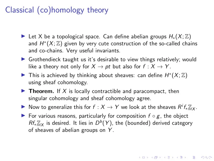
Classical (co)homology theory ◮ Let X be a topological space. Can define abelian groups H ∗ ( X ; Z ) and H ∗ ( X ; Z ) given by very cute construction of the so-called chains and co-chains. Very useful invariants. ◮ Grothendieck taught us it’s desirable to view things relatively; would like a theory not only for X → pt but also for f : X → Y . ◮ This is achieved by thinking about sheaves: can define H ∗ ( X ; Z ) using sheaf cohomology. ◮ Theorem. If X is locally contractible and paracompact, then singular cohomology and sheaf cohomology agree. ◮ Now to generalize this for f : X → Y we look at the sheaves R i f ∗ Z X . ◮ For various reasons, particularly for composition f ◦ g , the object Rf ∗ Z X is desired. It lies in D b ( Y ), the (bounded) derived category of sheaves of abelian groups on Y .
Poincar´ e duality ◮ In topology, it is desirable to intersect cycles. While this can be represented by cup product in cohomology, the most useful result is probably the Poincar´ e duality: If X is a compact orientable real n -dimensional manifold, then we have perfect pairing H ∗ ( X , Z ) × H n −∗ ( X , Z ) → H n ( X , Z ) ∼ = Z . ◮ When X is no longer a manifold, Poincar´ e duality no longer holds. On the other hand, it’s unclear how to intersect (co)chains in X nicely. ◮ Let us bring our attention to the case when X is an n -dimensional complex variety. So the non-smoothness of X may be studied as follows: we have a stratification X = X 2 n ⊃ X 2 n − 2 ⊃ ... ⊃ X 2 ⊃ X 0 such that each X 2 i − 2 ⊂ X 2 i is closed and each X 2 i − X 2 i − 2 is a topological orientable real manifold of dimension 2 i .
Intersection homology ◮ Goresky-MacPherson came up with the idea of intersection (co)homology, as follows: a k -chain C on X is allowable if C ∩ X 2 n − 2 i has dimension at most k − i − 1 for any i ≥ 1. ◮ Let IH ∗ ( X ; Q ) be the homology groups of the complex of allowable chains with allowable boundaries on X , called the intersection homology groups. Goresky-MacPherson showed that IH ∗ ( X ; Q ) does not depend on the choice of the stratification. ◮ For example let X be the nodal curve X = ( y 2 = x 3 − x 2 ) ⊂ CP 2 . We have H 1 ( X ; Q ) = Q . However, IH 1 ( X ; Q ) = 0 because an allowable 1-chain must not touch the singularity. ◮ We still have IH 2 ( X ; Q ) ∼ = IH 0 ( X ; Q ) ∼ = Q , so the intersection homology of X is the same as the ordinary homology its normalization ˜ X ∼ = CP 1 . In fact there is always a natural isomorphism IH ∗ ( X ; Q ) ∼ = H ∗ ( ˜ X ; Q ) for any algebraic curve X . ◮ Theorem. Suppose X is proper. We have a perfect pairing IH ∗ ( X ; Q ) × IH 2 n −∗ ( X ; Q ) → IH 2 n ( X ; Q ) = H 2 n ( X ; Q ) ∼ = Q for coefficients in Q .
Perverse sheaves We have again a perfect pairing Theorem. IH ∗ ( X ; Q ) × IH 2 n −∗ ( X ; Q ) → IH 2 n ( X ; Q ) = H 2 n ( X ; Q ) ∼ = Q for coefficient in Q . ◮ As we saw to have (co)homology theory relatively (for X → Y rather than X → pt ) we would like a sheaf version. With Goresky and MacPherson, Deligne worked out the sheaf version: there exists a subcategory Perv( X ) of the bounded derived category D b ( X ) of sheaves of Q -vector spaces on X , called the subcategory of perverse sheaves. ◮ Perv( X ) is the full subcategory of D b ( X ) whose objects are those F such that 1. dim R supp( H − k ( F )) ≤ 2 k (in particular is empty if k < 0). 2. dim R supp( H − k ( D X F )) ≤ 2 k , for the Verdier dual D X F of F . ◮ The category Perv( X ) can be proved to have an object IC X whose restriction to the smooth part X ′ := X 2 n − X 2 n − 2 of X is just Q X ′ [ n ], and such that there is a canonical isomorphism IH n −∗ ( X ; Q ) ∼ = H ∗ ( X ; IC X ). ◮ In fact, IC X can be characterized as the unique simple object in Perv( X ) with this property. ◮ The Poincar´ e duality can be interpreted as that IC X is Verdier self-dual.
An abelian category Perv( X ) is the full subcategory of D b ( X ) whose objects are those F such that 1. dim supp( H − k ( F )) ≤ k (in particular H k ( F ) is trivial for k > 0). 2. dim supp( H − k ( D X F )) ≤ k , for the Verdier dual D X F of F . ◮ The category D b ( X ) is an additive category that is basically never abelian; because the non-abelian-ness of D b ( X ) reflects why Sh( X ) (the category of sheaves of Q -vector spaces on X ) has to be derived. ◮ Miracle happens, that the subcategory Perv( X ) is abelian! ◮ Well, I guess the idea is really that Perv( X ) is secretly a way to modify the abelian category Sh( X ). In fact, the bounded derived category of Perv( X ) is again D b ( X ). ◮ The fact that the category Perv( X ) is abelian is somewhat behind its numerous applications in representation theory, typically in the form of equivalences of category that for some stack X we have Perv( X ) = some abelian category of representations or characters .
That Perv( X ) is great for representation theory Perv( X ) = some abelian category of representations or characters. (This slide is a supplement and is not needed for future slides.) ◮ Basically, representation theory studies how non-commutative a group and/or algebra is. In a twisted sense it attaches invariants to groups/algebras that detect how non-commutative they are. ◮ On the other hand, consider for an algebraic group G the quotient stack [ G / G ] where G acts on G by conjugation. That G is non-commutative is reflected by how different element in G have different centralizer, or how stacky [ G / G ] is. ◮ This gives a reason, at heuristically, how Perv([ G / G ]) detects representation theory of G . ◮ This is particularly fruitful for representation theory of G ( F q ) where G is a reductive group over a finite field F q ; Lusztig describes G ( F q ) via various subcategories of Perv([ G / G ]).
Another example: Geometric Satake Perv( X ) = some abelian category of representations or characters. (This slide is a supplement and is not needed for future slides.) ◮ Let G be a connected reductive group over C . Consider LG = Hom(Spec C (( t )) , G ) the loop group and L + G = Hom(Spec C [[ t ]] , G ) the arc group. Then we have an equivalence of category Perv( L + G \ LG / L + G ) = Rep( G ∨ ) where G ∨ is the dual reductive group (a reductive group over C whose combinatorial datum is opposite to that of G ). This is the Geometric Satake, and is of fundamental importance to Langlands program as Perv( L + G \ LG / L + G ) describes representations of LG with a fixed L G -vector. In the mixed characteristic setting, it’s representations of G ( Q p ) with a G ( Z p )-fixed vector.
A toy example in Minimal Model Program ◮ In minimal model program for 3-folds, Mori connected minimal models with flops. ◮ A flop is a pair of birational proper surjections: X Y Z of 3-folds with certain properties. In particular, X and Y are similar to being smooth (terminal singularity) and we will pretend they are smooth. ◮ The morphisms f , g are small contractions; outside a few curves on X and Y and a few points on Z they are isomorphic, and the preimage of a point in Z is at worst curves. ◮ In general, a morphism f : X → Z to an equi-dimensional variety Z is called small to representation theorists (not algebraic geometers unless dim Z = 3) if codim { z ∈ Z | dim f − 1 ( z ) ≥ i } ≥ 2 i + 1. ◮ Do you agree this looks like a relative version of allowable chains?
A toy example in Minimal Model Program, cont. codim { y ∈ Y | dim f − 1 ( y ) ≥ i } ≥ 2 i + 1. Do you agree this looks like a relative version of allowable chains? ◮ It is indeed the case that the machinery of perverse sheaves is able to treat small proper morphisms as if they are smooth of dimension 0, i.e. ´ etale. ◮ Birational ´ etale morphisms are isomorphisms. For us this means we have Rf ∗ IC X = IC Z = Rg ∗ IC Y . But X and Y are (almost) smooth! We have H ∗ ( X ; Q ) = H ∗ ( Z ; Rf ∗ Q X ) = H ∗ ( Z ; Rf ∗ IC X [ − 3]) = H ∗ ( Z ; IC Z [ − 3]) = IH ∗ ( Z ; Q ) . ◮ Same for Y , so H ∗ ( X ; Q ) = IH ∗ ( Z ; Q ) = H ∗ ( Y ; Q ). ◮ For Mori, this proved that birationally equivalent minimal models in 3d have isomorphic (co)homology groups in Q -coefficients. Sweet?
Recommend
More recommend
Explore More Topics
Stay informed with curated content and fresh updates.
