Chapter 13 Uncertainty Review of probability theory Probabilistic - PowerPoint PPT Presentation
Chapter 13 Uncertainty Review of probability theory Probabilistic reasoning Bayesian reasoning Bayesian Belief Networks (BBNs) 1 Probability Theory The nonmonotonic logics we covered introduce a mechanism for the systems to believe in
Chapter 13 Uncertainty Review of probability theory Probabilistic reasoning Bayesian reasoning Bayesian Belief Networks (BBNs) 1
Probability Theory The nonmonotonic logics we covered introduce a mechanism for the systems to believe in propositions (jump to conclusions) in the face of uncertainty. When the truth value of a proposition p is unknown, the system can assign one to it based on the rules in the KB. Probability theory takes this notion further by allowing graded beliefs. In addition, it provides a theory to assign beliefs to relations between propositions (e.g., p ∧ q), and related propositions (the notion of dependency). 2
Probabilities for propositions We write probability(A) ,or frequently P(A) in short, to mean the “probability of A.” But what does P(A) mean? P(I will draw ace of hearts) P(the coin will come up heads) P(it will snow tomorrow) P(the sun will rise tomorrow) P(the problem is in the third cylinder) P(the patient has measles) 3
Frequency interpretation • Draw a card from a regular deck: 13 hearts, 13 spades, 13 diamonds, 13 clubs. Total number of cards = n = 52 = h + s + d + c. • The probability that the proposition A=“the card is a hearts” is true corresponds to the relative frequency with which we expect to draw a hearts. P(A) = h / n 4
Frequency interpretation (cont’d) • The probability of an event A is the occurrences where A holds divided by all the possible occurrences: P(A) = #A holds / #total • P (I will draw ace of hearts ) ? • P (I will draw a spades) ? • P (I will draw a hearts or a spades) ? • P (I will draw a hearts and a spades) ? 5
Definitions • An elementary event or atomic event is a happening or occurrence that cannot be made up of other events. • An event is a set of elementary events. • The set of all possible outcomes of an event E is the sample space or universe for that event. • The probability of an event E in a sample space S is the ratio of the number of elements in E to the total number of possible outcomes of the sample space S of E. Thus, P(E) = |E| / |S|. 6
Subjective interpretation • There are many situations in which there is no objective frequency interpretation: • On a cold day, just before letting myself glide from the top of Mont Ripley, I say “there is probability 0.2 that I am going to have a broken leg”. • You are working hard on your AI class and you believe that the probability that you will get an A is 0.9. • The probability that proposition A is true corresponds to the degree of subjective belief. 7
Axioms of probability • There is a debate about which interpretation to adopt. But there is general agreement about the underlying mathematics. • Values for probabilities should satisfy the three basic requirements: • 0 ≤ P(A) ≤ 1 • P(A ∨ B) = P(A) + P(B) • P(true) = 1 8
Probabilities must lie between 0 and 1 • Every probability P(A) must be positive, and between 0 and 1, inclusive: 0 ≤ P(A) ≤ 1 • In informal terms it simply means that nothing can have more than a 100% chance of occurring or less than a 0% chance 9
Probabilities must add up • Suppose two events are mutually exclusive i.e., only one can happen, not both • The probability that one or the other occurs is then the sum of the individual probabilities • Mathematically, if A and B are disjoint, i.e., ¬ (A ∧ B) then: P(A ∨ B) = P(A) + P(B) • Suppose there is a 30% chance that the stock market will go up and a 45% chance that it will stay the same. It cannot do both at once, and so the probability that it will either go up or stay the same must be 75%. 10
Total probability must equal 1 • Suppose a set of events is mutually exclusive and collectively exhaustive. This means that one (and only one) of the possible outcomes must occur • The probabilities for this set of events must sum to 1 • Informally, if we have a set of events that one of them has to occur, then there is a 100% chance that one of them will indeed come to pass • Another way of saying this is that the probability of “always true” is 1: P(true) = 1 11
These axioms are all that is needed • From them, one can derive all there is to say about probabilities. • For example we can show that: • P( ¬ A) = 1 - P(A) because P(A ∨ ¬ A) = P (true) by logic P(A ∨ ¬ A) = P(A) + P( ¬ A) by the second axiom P(true) = 1 by the third axiom P(A) + P( ¬ A) = 1 combine the above two • P(false) = 0 because false = ¬ true by logic P(false) = 1 - P(true) by the above 12
Graphic interpretation of probability B A • A and B are events • They are mutually exclusive: they do not overlap, they cannot both occur at the same time • The entire rectangle including events A and B represents everything that can occur • Probability is represented by the area 13
Graphic interpretation of probability (cont’d) C B A • Axiom 1: an event cannot be represented by a negative area. An event cannot be represented by an area larger than the entire rectangle • Axiom 2: the probability of A or B occurring must be just the sum of the probability of A and the probability of B • Axiom 3: If neither A nor B happens the event shown by the white part of the rectangle (call it C) must happen. There is a 100% chance that A, 14 or B, or C will occur
Graphic interpretation of probability (cont’d) B B • P( ¬ B) = 1 – P(B) • because probabilities must add to 1 15
Graphic interpretation of probability (cont’d) B A • P(A ∨ B) = P(A) + P(B) - P(A ∧ B) • because the intersection area is counted twice 16
Random variables • The events we are interested in have a set of possible values. These values are mutually exclusive , and exhaustive . • For example: coin toss: {heads, tails} roll a die: {1, 2, 3, 4, 5, 6} weather: {snow, sunny, rain, fog} measles: {true, false} • For each event, we introduce a random variable which takes on values from the associated set. Then we have: P(C = tails) rather than P(tails) P(D = 1) rather than P(1) P(W = sunny) rather than P(sunny) P(M = true) rather than P(measles) 17
Probability Distribution A probability distribution is a listing of probabilities for every possible value a single random variable might take. For example: 1/6 weather prob. 1/6 snow 0.2 sunny 0.6 1/6 1/6 rain 0.1 fog 0.1 1/6 1/6 18
Joint probability distribution A joint probability distribution for n random variables is a listing of probabilities for all possible combinations of the random variables. For example: Construction Traffic Probability True True 0.3 True False 0.2 False True 0.1 False False 0.4 19
Joint probability distribution (cont’d) Sometimes a joint probability distribution table looks like the following. It has the same information as the one on the previous slide. ¬ Construction Construction Traffic 0.3 0.1 ¬ Traffic 0.2 0.4 20
Why do we need the joint probability table? It is similar to a truth table, however, unlike in logic, it is usually not possible to derive the probability of the conjunction from the individual probabilities. This is because the individual events interact in unknown ways. For instance, imagine that the probability of construction (C) is 0.7 in summer in Houghton, and the probability of bad traffic (T) is 0.05. If the “construction” that we are referring to in on the bridge, then a reasonable value for P(C ∧ T) is 0.6. If the “construction” we are referring to is on the sidewalk of a side street, then a reasonable value for P(C ∧ T) is 0.04. 21
Why do we need the joint probability table? (cont’d) P(A ∧ B) = 0 A B P(A ∧ B) = n A B P(A ∧ B) = m m>n A B 22
Marginal probabilities ¬ Construction Construction Traffic 0.3 0.1 0.4 ¬ Traffic 0.2 0.4 0.6 0.5 0.5 1.0 What is the probability of traffic, P(traffic)? P(traffic ∧ construction) + P(traffic) = P(traffic ∧ ¬ construction) = 0.3 + 0.1 = 0.4 Note that the table should be consistent with respect to the axioms of probability: the values in the whole table should add up to 1; for any event A, P(A) should be 1 - P( ¬ A); and so on. 23
More on computing probabilities ¬ Construction Construction Traffic 0.3 0.1 0.4 ¬ Traffic 0.2 0.4 0.6 0.5 0.5 1.0 • Given the joint probability table, we have all the information we need about the domain. We can calculate the probability of any logical formula • P(traffic ∨ construction) = 0.3 + 0.1 + 0.2 = 0.6 • P( construction → traffic) = P ( ¬ construction ∨ traffic) by logic = 0.1 + 0.4 + 0.3 = 0.8 24
Dynamic probabilistic KBs Imagine an event A. When we know nothing else, we refer to the probability of A in the usual way: P(A). If we gather additional information, say B, the probability of A might change. This is referred to as the probability of A given B: P(A | B). For instance, the “general” probability of bad traffic is P(T). If your friend comes over and tells you that construction has started, then the probability of bad traffic given construction is P(T | C). 25
Prior probability The prior probability ; often called the unconditional probability , of an event is the probability assigned to an event in the absence of knowledge supporting its occurrence and absence, that is, the probability of the event prior to any evidence. The prior probability of an event is symbolized: P (event). 26
Recommend
More recommend
Explore More Topics
Stay informed with curated content and fresh updates.
