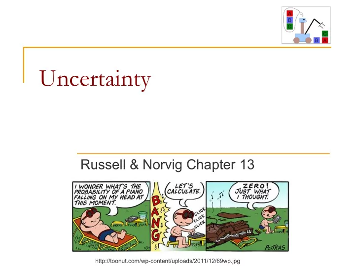

Uncertainty Russell & Norvig Chapter 13 http://toonut.com/wp-content/uploads/2011/12/69wp.jpg
Uncertainty Let A t be the action of leaving for the airport t minutes before your flight Will A t get you there on time? Uncertainty results from: partial observability (road state, other drivers' plans, etc.) 1. noisy sensors (traffic reports) 2. uncertainty in action outcomes (flat tire, etc.) 3. complexity of modeling traffic 4.
Uncertainty Let A t be the action of leaving for the airport t minutes before your flight Will A t get you there on time? A purely logical approach either risks falsehood: “ A 120 will get me there on time”, or 1. leads to conclusions that are too weak for decision 2. making: “ A 120 will get me there on time if there's no accident and it doesn't rain and my tires remain intact etc.” ( A 1440 might reasonably be said to get me there on time but I'd have to stay overnight in the airport … )
Questions n How to represent uncertainty in knowledge? n How to perform inference with uncertain knowledge? n Which action to choose under uncertainty?
Dealing with uncertainty n Implicit q Ignore what you are uncertain of when you can q Build procedures that are robust to uncertainty n Explicit q Build a model of the world that describes uncertainty about its state, dynamics, and observations q Reason about the effect of actions given the model
Methods for handling uncertainty n Default Reasoning: q Assume the car does not have a flat tire q Assume A 120 works unless contradicted by evidence n Issues: What assumptions are reasonable? How to handle contradictions? n Worst case reasoning (the world behaves according to Murphy’s law). n Probability q Model agent's degree of belief q Given the available evidence, A 120 will get me there on time with probability 0.95
Probability n Probabilities relate propositions to agent's own state of knowledge e.g., P(A 120 | no reported accidents) = 0.96 n Probabilities of propositions change with new evidence: e.g., P(A 120 | no reported accidents, 5 a.m.) = 0.99
Making decisions under uncertainty Suppose I believe the following: P(A 60 gets me there on time | … ) = 0.001 P(A 90 gets me there on time | … ) = 0.70 P(A 120 gets me there on time | … ) = 0.95 P(A 150 gets me there on time | … ) = 0.99 P(A 1440 gets me there on time | … ) = 0.9999 n Which action to choose? Depends on my preferences for missing flight vs. time spent waiting, etc. q Utility theory is used to represent and infer preferences q Decision theory = probability theory + utility theory
Axioms of probability n For any events A, B in a space of events Ω q 0 ≤ P( A ) ≤ 1 q P( Ω ) = 1 and P( φ ) = 0 q P( A ∨ B ) = P( A ) + P( B ) - P( A ∧ B ) Ω
Axioms of probability ∑ P ( ω ) = 1 q 0 ≤ P( ω ) ≤ 1 ω ∈Ω q P(A ∨ B) = P(A) + P(B) - P(A ∧ B) [inclusion-exclusion principle] Ω
Example n You draw a card from a deck of cards (52 cards). What is the probability of each of the following events: q A king q A face card q A spade q A face card or a red suit q A card
Where do probabilities come from Two camps: n Frequentist interpretation n Bayesian interpretation
Frequentist interpretation n Draw a ball from an urn containing n balls of the same size; r are red, the rest black. n The probability of the event “the ball is red” corresponds to the relative frequency with which we expect to draw a red ball P(red) = ?
Subjective probabilities There are many situations in which there is no objective frequency interpretation: q E.g. the probability that you will get to the airport in time. q There are theoretical justifications for subjective probabilities!
The Bayesian viewpoint n Probability is "degree-of-belief”. n To the Bayesian, probability lies subjectively in the mind, and can be different for people with different information n In contrast, to the frequentist, probability lies objectively in the external world.
Random Variables n A random variable can be thought of as an unknown value that may change every time it is inspected. n Suppose that a coin is tossed three times and the sequence of heads and tails is noted. The event space for this experiment is: S={HHH, HHT, HTH, HTT, THH, THT, TTH, TTT}. X - the number of heads in three coin tosses. X assigns each outcome in S a number from the set {0, 1, 2, 3}. Outcome HHH HHT HTH THH HTT THT TTH TTT X 3 2 2 2 1 1 1 0 n We can now ask the question – what is the probability for observing a particular value for X (the distribution of X).
Random Variables n Boolean random variables e.g., Cavity (do I have a cavity?) Distribution characterized by a number p. n Discrete random variables e.g., Weather is one of < sunny,rainy,cloudy,snow > n Domain values must be exhaustive and mutually exclusive n The (probability) distribution of a random variable X with m values x 1 , x 2 , … , x n is: (p 1 , p 2 , … , p m ) with P(X=x i ) = p i and Σ i p i = 1
Joint Distribution n Given n random variables X 1 , … , X n n The joint distribution of these variables is a table in which each entry gives the probability of one combination of values of X 1 , … ,X n n Example: Toothache ¬ Toothache Cavity 0.04 0.06 ¬ Cavity 0.01 0.89 P(Cavity ∧ ¬ Toothache) P( ¬ Cavity ∧ Toothache)
It’s all in the joint Toothache ¬ Toothache Cavity 0.04 0.06 ¬ Cavity 0.01 0.89 n P( Toothache ) = P( (Toothache ∧ Cavity) v (Toothache ∧ ¬ Cavity) ) = P( Toothache ∧ Cavity ) + P( Toothache ∧ ¬ Cavity ) = 0.04 + 0.01 = 0.05 We summed over all values of Cavity: marginalization n P( Toothache v Cavity ) = P( (Toothache ∧ Cavity) v (Toothache ∧ ¬ Cavity) v ( ¬ Toothache ∧ Cavity) ) = 0.04 + 0.01 + 0.06 = 0.11 These are examples of inference by enumeration
Conditional Probability n Definition: P(A|B) =P(A ∧ B) / P(B) (if P(B) > 0) n Read: probability of A given B q Example: P(snow) = 0.03 but P(snow | winter) = 0.06, P(snow | summer) = 1e-4 n can also write this as: P(A ∧ B) = P(A|B) P(B) n called the product rule
Example Toothache ¬ Toothache Cavity 0.04 0.06 ¬ Cavity 0.01 0.89 P(Cavity|Toothache) = P(Cavity ∧ Toothache) / P(Toothache) = 0.04/0.05 = 0.8
Independence n Events A and B are independent if P(A | B) = P(A) which is equivalent to: P(A ∧ B) = P(A) P(B) q Example: the outcomes of rolling two dice are independent.
Bayes’ Rule P(A ∧ B) = P(A|B) P(B) = P(B|A) P(A) P(B|A) = P(A|B) P(B) P(A) Image from: http://commons.wikimedia.org/wiki/File:Thomas_Bayes.gif
Example Toothache ¬ Toothache n Given: Cavity 0.04 0.06 P(Cavity) = 0.1 ¬ Cavity 0.01 0.89 P(Toothache) = 0.05 P(Cavity|Toothache) = 0.8 n Using Bayes’ rule: P(Toothache|Cavity) = (0.8x0.05)/0.1 = 0.4
The Monty Hall Problem Suppose you're on a game show, and you're given the choice of three doors: Behind one door is a car; behind the others, goats. You pick a door, say No. 1, and the host, who knows what's behind the doors, opens another door, say No. 3, which has a goat. He then says to you, "Do you want to pick door No. 2?" Is it to your advantage to switch your choice? source: http://en.wikipedia.org/wiki/Monty_Hall_problem
Solution P(C2|O3) = P(O3|C2)P(C2)/P(O3) = = 1 * 1/3 / 1/2 = 2/3 P(C1|O3) = P(O3|C1)P(C1)/P(O3) = 1/2*1/3 / 1/2 = 1/3 Your pick Host opens Should you pick this one instead?
Solution P(C2|O3) = P(O3|C2)P(C2)/P(O3) = = 1 * 1/3 / 1/2 = 2/3 P(O3) = P(O3|C1)P(C1) + P(O3|C2)P(C2) + P(O3|C3)P(C3) = = 1/2*1/3 + 1*1/3 + 0*1/3 = 1/2
Probabilities in the wumpus world 1,4 2,4 3,4 4,4 1,3 2,3 3,3 4,3 There is no safe choice at this point! But are there squares that are less likely to contain a pit? 1,2 2,2 3,2 4,2 B OK 1,1 2,1 3,1 4,1 B OK OK
Probabilities in the wumpus world 1,4 2,4 3,4 4,4 1,3 2,3 3,3 4,3 There is no safe choice at this point! But are there squares that are less likely to contain a pit? 1,2 2,2 3,2 4,2 B OK 1,1 2,1 3,1 4,1 B OK OK 1,3 1,3 1,3 1,3 1,3 1,2 2,2 1,2 2,2 1,2 2,2 1,2 2,2 1,2 2,2 B B B B B OK OK OK OK OK 1,1 2,1 3,1 1,1 2,1 3,1 1,1 2,1 3,1 1,1 2,1 3,1 1,1 2,1 3,1 B B B B B OK OK OK OK OK OK OK OK OK OK 0.2 x 0.2 = 0.04 0.2 x 0.8 = 0.16 0.8 x 0.2 = 0.16 0.2 x 0.2 = 0.04 0.2 x 0.8 = 0.16
Generalization of Bayes’ rule P(A ∧ B ∧ C) = P(A ∧ B|C) P(C) = P(A|B,C) P(B|C) P(C) P(A ∧ B ∧ C) = P(A ∧ B|C) P(C) = P(B|A,C) P(A|C) P(C) P(B|A,C) = P(A|B,C) P(B|C) P(A|C)
It’s all in the joint but… n The naïve representation runs into problems. n Example: q Patients in a hospital are described by attributes such as: Background: age, gender, history of diseases, … n Symptoms: fever, blood pressure, headache, … n Diseases: pneumonia, heart attack, … n n A probability distribution needs to assign a number to each combination of values of these attributes q Size of table is exponential in number of attributes
Bayesian Networks n Provide an efficient representation that relies on independence relations between variables.
Product rule n P(A ∧ B ∧ C) = P(A|B,C) P(B|C) P(C)
Bayesian Networks P(B) P(E) Burglary Earthquake 0.001 0.002 B E P(A| … ) T T 0.95 Alarm T F 0.94 F T 0.29 F F 0.001 A P(J|A) A P(M|A) JohnCalls MaryCalls T 0.90 T 0.70 F 0.05 F 0.01
Recommend
More recommend