Chapter 1 Rationale for Survival Analysis Time-to-event data have - PDF document
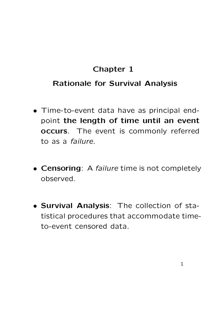
Chapter 1 Rationale for Survival Analysis Time-to-event data have as principal end- point the length of time until an event occurs . The event is commonly referred to as a failure . Censoring : A failure time is not completely observed.
Chapter 1 Rationale for Survival Analysis • Time-to-event data have as principal end- point the length of time until an event occurs . The event is commonly referred to as a failure . • Censoring : A failure time is not completely observed. • Survival Analysis : The collection of sta- tistical procedures that accommodate time- to-event censored data. 1
Example: AML study Below are preliminary results (1977) from a clinical trial to evaluate the efficacy of maintenance chemotherapy for acute myelogenous leukemia (AML). After reaching a status of remission through treatment by chemother- apy, the patients who entered the study were assigned randomly to two groups. The first group received main- tenance chemotherapy; the second, or control, group did not. The objective of the trial was to see if maintenance chemotherapy prolonged the time un- til relapse . Group Length of complete remission (in weeks) Maintained 9, 13, 13+, 18, 23, 28+, 31, 34, 45+, 48, 161+ Nonmaintained 5, 5, 8, 8, 12, 16+, 23, 27, 30, 33, 43, 45 The + indicates a censored value. 2
• Serious bias in estimated quantities, which lowers the efficacy of the study. a. Throw out censored observations. b. Treat censored observations as exact. c. Account for the censoring. η = median µ = mean 0.005 η µ η η µ µ 0.000 23 25.1 28 31 38.5 52.6 a a b c b c -0.005 20 30 40 50 weeks in remission 3
Basic Definitions & Identities The r.v. T denotes failure time with cdf F ( · ) and pdf f ( · ). cdf F ( · ): � t dF ( t ) F ( t ) = P ( T ≤ t ) = f ( x ) dx and = f ( t ) dt 0 That is, by definition of derivative, F ( t + ∆ t ) − F ( t ) P ( t < T ≤ t + ∆ t ) f ( t ) = lim = lim ∆ t ∆ t ∆ t → 0 + ∆ t → 0 + P ( t ≤ T < t + ∆ t ) and since T is a continuous r.v., = lim ∆ t ∆ t → 0 + Survivor function S ( · ): � ∞ S ( t ) = P ( T > t ) = 1 − F ( t ) = f ( x ) dx t At t = 0, S ( t ) = 1 and decreases to 0 as t increases to ∞ . We thus can express the pdf as f ( t ) = − dS ( t ) . dt 4
Hazard function h ( · ): P ( t ≤ T < t + ∆ t | T ≥ t ) = f ( t ) h ( t ) = lim ∆ t S ( t ) ∆ t → 0 + = − dS ( t ) /dt = − d log ( S ( t )) S ( t ) dt Of course, h ( t ) ≥ 0 at all times t . Cumulative hazard function H ( · ): � t H ( t ) = h ( u ) du = − log( S ( t )) 0 At t = 0, H ( t ) = 0 and increases to ∞ as t increases to ∞ . Hence, the relationship S ( t ) = exp ( − H ( t )) . 5
The hazard function h ( t ) • specifies the instantaneous rate of failure at T = t given that the individual survived up to time t . It measures the potential of failure in an instant at time t given the individual’s survival time reaches t . • is the slope of the tangent line to H ( t ) = − log ( S ( t )) at T = t • specifies the distribution of T 6
Cumulative Hazard H(t) 15.0 and tangent lines with slopes h(t) 12.5 10.0 H(t) = -log(S(t)) 3.00 7.5 5.0 ≈1.69 2.5 ≈ .57 ≈ .187 0.0 0 1 2 3 4 5 6 7 8 9 10 t 1.0 Survival Curve S(t) and 0.9 tangent lines with slopes -h(t)*S(t) -.165 0.8 0.7 0.6 S(t) 0.5 -.294 0.4 0.3 0.2 0.1 -.06 -.001 0.0 0 1 2 3 4 5 6 7 8 9 10 t 7
p th-quantile: The value t p such that F ( t p ) = P ( T ≤ t p ) = p. That is, t p = F − 1 ( p ). Also called the 100 × p th percentile . Mean Lifetime E ( T ): For random variable T ≥ 0, � ∞ E ( T ) = t · f ( t ) dt 0 � ∞ = S ( t ) dt. 0 total area under the survivor curve 8
Three Censoring Models Let T 1 , T 2 , . . . , T n be independent and identically distributed (iid) with distribution function (d.f.) F . Type I censoring: • In engineering applications, we test lifetimes of tran- sistors, tubes, chips, etc. • Put them all on test at time t = 0 and record their times to failure. Some items may take a long time to “burn out” and we do not want to wait that long to terminate the experiment. • Terminate the experiment at a prespecified time t c . • The number of observed failure times is random. If n is the number of items put on test, then we could observe 0 , 1 , 2 , . . . , n failure times. 9
The following illustrates a possible trial: The t c is a fixed censoring time. • We do not observe the T i , but do observe Y 1 , Y 2 , . . . , Y n where � T i if T i ≤ t c Y i = min( T i , t c ) = t c if t c < T i . • It is useful to introduce a binary random variable δ which indicates if a failure time is observed or censored, � 1 if T ≤ t c δ = 0 if t c < T . We then observe the iid random pairs ( Y i , δ i ). 10
Type II censoring: • In similar engineering applications as above, the ex- periment is run until a prespecified fraction r/n of the n items has failed. • Let T (1) , T (2) , . . . , T ( n ) denote the ordered values of the random sample T 1 , . . . , T n . By plan, the experiment is terminated after the r th failure occurs. We only observe the r smallest ob- servations in a random sample of n items. • For example, let n = 25 and take r = 15. When we observe 15 burn out times, we terminate the experiment. • The following illustrates a possible trial: Here the last 10 observations are assigned the value of T (15) . Hence, we have 10 censored observations. 11
• Notice that we could wait an arbitrarily long time to observe the 15th failure time as T (15) is random; or, we could see all 15 very early on. • More formally, we observe the following full sample. Y (1) = T (1) Y (2) = T (2) . . . . . . . . . Y ( r ) = T ( r ) Y ( r +1) = T ( r ) . . . . . . . . . Y ( n ) = T ( r ) . The data consist of the r smallest lifetimes T (1) , . . . , T ( r ) out of the n iid lifetimes T 1 , . . . , T n with continuous p.d.f f ( t ) and survivor function S ( t ). 12
Random Right Censoring: Random censoring occurs frequently in medical studies. In clinical trials, patients typically enter a study at dif- ferent times. Then each is treated with one of several possible therapies. We want to observe their ” failure ” time but censoring can occur in one of the following ways: 1. Loss to Follow-up . Patient moves away. We never see him again. We only know he has survived from entry date until he left. So his survival time is ≥ the observed value. 2. Drop Out . Bad side effects forces termination of treatment. Or patient refuses to continue treat- ment for whatever reasons. 3. Termination of Study . Patient is still “alive” at end of study. The following illustrates a possible trial: 13
------------------------------------------------------ T 1 1 T 2 ---------------- 2 T 3 ------------- 3 ......... 0 Study Study end start The AML study contain randomly right-censored data. Formally: Let T denote a lifetime with d.f. F and sur- vivor function S f and C denote a random censor time with d.f. G , p.d.f. g , and survivor function S g . Each in- dividual has a lifetime T i and a censor time C i . On each of n individuals we observe the pair ( Y i , δ i ) where � 1 if T i ≤ C i Y i = min( T i , C i ) and δ i = 0 if C i < T i . • We observe n iid random pairs ( Y i , δ i ). • The times T i and C i are usually assumed to be in- dependent. • This is a strong assumption. If a patient drops out because of complications with the treatment (case 2 above), it is clearly offended. 14
Remarks: • If the distribution of C does not involve any parame- ters of interest, then the form of the observed likeli- hood function is the same for these three censoring models . n � ( f ( y i )) δ i · ( S f ( y i )) 1 − δ i . L = i =1 Thus, regardless of which of the three types of censoring is present, the maximization process yields the same estimated quantities. • Here we see how censoring is incorporated to adjust the estimates. Each observed value is ( y i , δ i ). An indi- vidual’s contribution is either it pdf f ( y i ); or S f ( y i ) = P ( T > y i ), the probability of survival beyond its ob- served censored time y i . In the complete data setting, all δ i = 1; that is, there is no censoring. The likelihood then has the usual form n � L = f ( y i ) . i =1 15
Major Goals Goal 1. To estimate and interpret survivor and/or hazard functions from survival data. 1 1 S(t) S(t) 0 0 t t Goal 2. To compare survivor and/or hazard functions. 1 new method S(t) old method weeks 0 13 Goal 3. To assess the relationship of explanatory variables to survival time, especially through the use of formal mathematical modelling. 1.0 0.9 0.8 0.7 hazard 0.6 0.5 WOMEN MEN 0.4 0.3 0.2 0.1 0.0 0 10 20 30 40 50 60 70 age at diagnosis (years) 16
Chapter 2 Kaplan-Meier Estimator of Survivor Function I 1 I 2 · · · I i − 1 I i · · · | ———— | ————— | ———— | ——— | ——– | —— 0 y (1) y (2) y ( i − 1) y ( i ) The y ( i ) : i th distinct ordered censored or uncensored observation and right endpoint of the interval I i , i = 1 , 2 , . . . , n ′ ≤ n . • death is the generic word for the event of interest. In the AML study, a “relapse” (end of remission period) = “death” • Cohort is a group of people who are followed through- out the course of the study. • People at risk at the beginning of the interval I i are those people who survived (not dead, lost, or withdrawn) the previous interval I i − 1 . Let R ( t ) denote the risk set just before time t and let 17
Recommend
More recommend
Explore More Topics
Stay informed with curated content and fresh updates.
