Central Limit Theorem Learning Objectives At the end of this - PowerPoint PPT Presentation
Chapter 7.4 & 7.5 Sampling Distributions and the Central Limit Theorem Learning Objectives At the end of this lecture, the student should be able to: State the statistical notation for parameters and statistics for two measures of
Chapter 7.4 & 7.5 Sampling Distributions and the Central Limit Theorem
Learning Objectives At the end of this lecture, the student should be able to: • State the statistical notation for parameters and statistics for two measures of variation. • Name one type of inference and describe it. • Explain the difference between a frequency distribution and sampling distribution • Describe the Central Limit Theorem in either words or formulas. • Describe how to calculate standard error
Introduction • Parameters, Statistics, and Inferences • Introduction to Sampling Distribution • Central Limit Theorem • Finding Probabilities Regarding X-bar Photograph by David Hawgood
Parameters, Statistics, and Inferences Review and Overview
Reminder of Statistic and Parameter • A statistic is a numerical measure describing a sample . Statistic Photographs by Che and Sandstein
Reminder of Statistic and Parameter Parameter • A statistic is a numerical measure describing a sample . Statistic • A parameter is a numerical measure describing a population . Photographs by Che and Sandstein
Notation of Statistics and Parameters Mea Measur sure Sta Statisti tistic Par arame ameter ter μ (mu) Mean x (x-bar) Ϭ 2 (sigma s 2 Variance squared) Standard Ϭ (sigma) s Deviation ^ Proportion p (p-hat) p
Inferences Photograph by Tomasz Sienicki
Inferences Photograph by Tomasz Sienicki
Types of Inferences 1. Estimation: we estimate the value of a population parameter using a sample
Types of Inferences 1. Estimation: we estimate the value of a population parameter using a sample ***We will practice this in Chapter 8***
Types of Inferences 1. Estimation: we estimate the value of a population parameter using a sample 2. Testing: we do a test to help us make a decision about a population parameter
Types of Inferences 1. Estimation: we estimate the value of a population parameter using a sample 2. Testing: we do a test to help us make a decision about a population parameter ***Chapter 9***
Types of Inferences 1. Estimation: we estimate the value of a population parameter using a sample 2. Testing: we do a test to help us make a decision about a population parameter 3. Regression: we make predictions or forecasts about a statistic
Types of Inferences 1. Estimation: we estimate the value of a population parameter using a sample 2. Testing: we do a test to help us make a decision about a population parameter 3. Regression: we make predictions or forecasts about a statistic ***We already did this in Chapter 4.2***
Types of Inferences 1. Estimation: we estimate the value of a population parameter using a sample 2. Testing: we do a test to help us make a decision about a population parameter 3. Regression: we make predictions or forecasts about a statistic Requires understanding sampling distributions and the Central Limit Theorem
Introduction to Sampling Distribution Different from Frequency Distribution
Frequency vs. Sampling Distribution Frequenc equency D y Dist istribut ribution ion Sampling Dist Sampling Distribut ribution ion 1. Make a histogram of a quantitative variable. 2. Draw the shape and name the distribution. 30 20 10 0
Frequency vs. Sampling Distribution Frequenc equency D y Dist istribut ribution ion Sampling Distribut Sampling Dist ribution ion 1. Start with a population. 1. Make a histogram of a 2. Decide on an n. quantitative variable. 3. Take as many samples of n 2. Draw the shape and as possible from the name the distribution. population. 30 4. Make an x-bar for each 20 sample. 10 5. Make a histogram of all the x- 0 bars.
Explanation of Sampling Distribution Sampling Dist Sampling Distribut ribution ion 1. Start with a population. 2. Decide on an n. 3. Take as many samples of n as possible from the population. 4. Make an x-bar for each sample. 5. Make a histogram of all the x- bars.
Explanation of Sampling Distribution Sampling Dist Sampling Distribut ribution ion 1. Start with a population. n=5 2. Decide on an n. 3. Take as many samples of n as possible from the population. 4. Make an x-bar for each sample. 5. Make a histogram of all the x- bars.
Explanation of Sampling Distribution x-bar = 23 Sampling Dist Sampling Distribut ribution ion 1. Start with a population. n=5 2. Decide on an n. 3. Take as many samples of n as possible from the population. 4. Make an x-bar for each sample. 5. Make a histogram of all the x- bars.
Explanation of Sampling Distribution x-bar = 23 Sampling Dist Sampling Distribut ribution ion 1. Start with a population. n=5 2. Decide on an n. 3. Take as many samples of n as possible from the population. 4. Make an x-bar for each sample. 5. Make a histogram of all the x- bars. x-bar = 21
Explanation of Sampling Distribution x-bar = 23 Sampling Dist Sampling Distribut ribution ion 1. Start with a population. n=5 2. Decide on an n. 3. Take as many samples of n as possible from the population. 4. Make an x-bar for each sample. 5. Make a histogram of all the x- bars. x-bar = 21 x-bar = 25
Explanation of Sampling Distribution Sampling Dist Sampling Distribut ribution ion Clas Class s Limit Limits s Frequenc equency of y of of of BM BMI x-bar bars 1. Start with a population. n=5 2. Decide on an n. BMI <20 2,626,094 3. Take as many samples of n BMI 20-<25 10,758,762 as possible from the BMI 25-<30 13,554,687 population. BMI 30-<35 12,605,250 4. Make an x-bar for each BMI 35-<40 9,300,551 sample. BMI >40 3,676,531 5. Make a histogram of all the x- Total 52,521,875 bars.
Explanation of Sampling Distribution Sampling Dist Sampling Distribut ribution ion 16,000,000 14,000,000 1. Start with a population. 12,000,000 n=5 2. Decide on an n. 10,000,000 8,000,000 3. Take as many samples of n 6,000,000 as possible from the 4,000,000 population. 2,000,000 0 4. Make an x-bar for each sample. 5. Make a histogram of all the x- bars.
Definition of a Sampling Distribution • A sampling distribution is a 16,000,000 probability distribution of a 14,000,000 sample statistic based on all 12,000,000 10,000,000 possible simple random 8,000,000 samples of the same size from 6,000,000 the same population . 4,000,000 2,000,000 0
Definition of a Sampling Distribution • A sampling distribution is a 16,000,000 probability distribution of a 14,000,000 sample statistic based on all 12,000,000 10,000,000 possible simple random 8,000,000 samples of the same size from 6,000,000 the same population . 4,000,000 2,000,000 • In the next section, we will talk 0 about the Central Limit Theorem, which is a proof that shows how we can use a sampling distribution for inference.
Central Limit Theorem Using it for Statistical Inference
Central Limit Theorem: In Words 16,000,000 For any normal distribution: 14,000,000 1. The sampling distribution 12,000,000 10,000,000 (the distributions of x-bars 8,000,000 from all possible samples) 6,000,000 is also a normal distribution 4,000,000 2,000,000 2. The mean of the x-bars is 0 actually µ 3. The standard deviation of the x-bars is actually σ/√n
Central Limit Theorem: In Formulas ….where µ x-bars =µ • n is the sample size σ x-bars =σ/√n • µ is the mean of the x distribution (population mean), and • σ is the standard x-bar - µ x-bars x-bar - µ z= = deviation of the x σ x-bars σ/√n distribution (population standard deviation)
Central Limit Theorem: In Formulas ….where µ x-bars =µ • n is the sample size σ x-bars =σ/√n • Note: Only works when n≥30! • µ is the mean of the x distribution (population z= = mean), and x-bar - µ x-bars x-bar - µ • σ is the standard σ x-bars σ/√n deviation of the x distribution (population standard deviation) The standard error is the standard deviation of the sampling distribution. For the x- bar sampling distribution, standard error (SE) = σ/√ n
Central Limit Theorem 30 1. If the distribution of x is x distribution normal, then the 20 distribution of x-bar is 10 also normal. 0 20,000,000 x-bar distribution 10,000,000 0
Central Limit Theorem 1. If the distribution of x is 30 x distribution normal, then the 20 distribution of x-bar is also normal. 10 2. Even if the distribution of x 0 is NOT normal, as long as n≥ 30, the Central Limit 20,000,000 Theorem says that the x- x-bar distribution bar distribution is 10,000,000 approximately normal. 0
Central Limit Theorem 1. If the distribution of x is 30 x distribution normal, then the 20 distribution of x-bar is also normal. 10 2. Even if the distribution of x 0 is NOT normal, as long as n≥ 30, the Central Limit 20,000,000 Theorem says that the x- x-bar distribution bar distribution is 10,000,000 approximately normal. 0 A sample statistic is considered unbiased if the mean of its sampling distribution equals the parameter being estimated.
Finding Probabilities Regarding X- bar Applying the Central Limit Theorem
Recommend
More recommend
Explore More Topics
Stay informed with curated content and fresh updates.
