Ce Central Li Limit The heorem number of measurements needed - PowerPoint PPT Presentation
Ce Central Li Limit The heorem number of measurements needed to estimate the mean convergence of the est estim imated ed m mean ean a better approximation than the Chebyshev Inequality (LLN). Xingru Chen
Ce Central Li Limit The heorem number of measurements needed to § estimate the mean convergence of the est estim imated ed m mean ean § a better approximation than the § Chebyshev Inequality (LLN). Xingru Chen xingru.chen.gr@dartmouth.edu XC 2020
Central Limit Theorem 𝑌 ! 𝑌 " 𝑌 # 𝑌 $ + ⋯ 𝑌 % + + + 𝑌 & 𝑌 ' + no normal density funct ction on XC 2020
Central Limit Theorem 𝑌 ! 𝑌 " 𝑌 # 𝑌 $ If 𝑇 ' is the sum of 𝑜 mutually independent random variables, then the distribution function of + ⋯ 𝑇 ' is well-approximated by a 𝑌 % + + normal density function. + 𝑌 & 𝑌 ' + no normal density de function XC 2020
CENT NTRAL LIMI MIT THE HEOR OREM M FOR OR BE BERNOU NOULLI TRIALS binomial distribution XC 2020
Bernoulli Trials A Bernou oulli trials proce ocess is a sequence of 𝑜 chance experiments such that § Each experiment has two pos ossibl ble ou outcom comes , which we may call success and failure. § The probability 𝑞 of success on each experiment is the same for each experiment, and this probability is not a ff ected by any knowledge of previous outcomes. The probability 𝑟 of failure is given by 𝑟 = 1 − 𝑞 . Wheel of Fortune Toss a Coin 12 12.5% 50% 50% 50 points & others head & tail Weather Forecast 𝒒 Bernoulli Trials 60% 60% not rain & rain outcome 1 & 2 XC 2020
Binomial Distribution § Let 𝑜 be a positive integer and let 𝑞 be a real number between 0 and 1. § Let 𝐶 be the random variable which counts the number of successes in a Ber Bernoulli trials proce ocess with parameters 𝑜 and 𝑞 . § Then the distribution 𝑐(𝑜, 𝑞, 𝑙) of 𝐶 is called the binomial distribution. 1 2 3 4 5 Bin Binomia ial Dist D istrib ibutio ion 𝑐 𝑜, 𝑞, 𝑙 = 𝑜 𝑙 𝑞 ( 𝑟 ')( ✗ ✓ ✗ ✗ ✓ XC 2020
Binomial Distribution § Consider a Bernoulli trials process with probability 𝑞 for success on each trial. § Let 𝑌 * = 1 or 0 according as the 𝑗 th outcome is a success or failure. § Let 𝑇 ' = 𝑌 & + 𝑌 % + ⋯ + 𝑌 ' . Then 𝑇 ' is the number of successes in 𝑜 trials. § We know that 𝑇 ' has as its distribution the binomial probabilities 𝑐(𝑜, 𝑞, 𝑙) . XC 2020
𝑜 increases drifts off to the right fl atten out XC 2020
The Standardized Sum of 𝑇 4 § Consider a Bernoulli trials process with probability 𝑞 for success on each trial. § Let 𝑌 * = 1 or 0 according as the 𝑗 th outcome is a success or failure. § Let 𝑇 ' = 𝑌 & + 𝑌 % + ⋯ + 𝑌 ' . Then 𝑇 ' is the number of successes in 𝑜 trials. § We know that 𝑇 ' has as its distribution the binomial probabilities 𝑐(𝑜, 𝑞, 𝑙) . § The standardized sum of 𝑇 ' is given by ∗ = , ! )'- '-. . 𝑇 ' 𝜏 % = ⋯ 𝜈 = ⋯ XC 2020
The Standardized Sum of 𝑇 4 § Consider a Bernoulli trials process with probability 𝑞 for success on each trial. § Let 𝑌 * = 1 or 0 according as the 𝑗 th outcome is a success or failure. § Let 𝑇 ' = 𝑌 & + 𝑌 % + ⋯ + 𝑌 ' . Then 𝑇 ' is the number of successes in 𝑜 trials. § We know that 𝑇 ' has as its distribution the binomial probabilities 𝑐(𝑜, 𝑞, 𝑙) . § The standardized sum of 𝑇 ' is given by ∗ = , ! )'- '-. . 𝑇 ' 𝜈 = 0 ∗ always has expected value 0 and variance 1 . § 𝑇 ' 𝜏 % = 1 XC 2020
The Standardized Sum of 𝑇 4 ∗ = 𝑇 ' − 𝑜𝑞 𝑐(𝑜, 𝑞, 𝑙) = 𝑇 ' 𝑜𝑞𝑟 𝑙 0 1 2 3 4 5 … 𝑜 ⋯ 𝑐(𝑜, 𝑞, 4) 𝑐(𝑜, 𝑞, 3) 𝑐(𝑜, 𝑞, 5) 𝑐(𝑜, 𝑞, 2) 𝑐(𝑜, 𝑞, 1) 𝑐(𝑜, 𝑞, 0) 𝑐(𝑜, 𝑞, 𝑜) 𝑜 − 𝑜𝑞 0 − 𝑜𝑞 1 − 𝑜𝑞 2 − 𝑜𝑞 3 − 𝑜𝑞 4 − 𝑜𝑞 5 − 𝑜𝑞 … 𝑦 𝑜𝑞𝑟 𝑜𝑞𝑟 𝑜𝑞𝑟 𝑜𝑞𝑟 𝑜𝑞𝑟 𝑜𝑞𝑟 𝑜𝑞𝑟 XC 2020
∗ = 𝑇 ' − 𝑜𝑞 𝑇 ' 𝑜𝑞𝑟 𝜈 = 0 𝜏 % = 1 XC 2020
standardized sum standard normal distribution shapes: same heights: di ff erent why? XC 2020
standard normal standardized sum distribution shapes: same why? heights: di ff erent standardized sum: ∑ (/0 ' ℎ * = 1 standard normal distribution 21 𝑔 𝑦 𝑒𝑦 = 1 : ∫ )1 XC 2020
' standardized sum: ∑ (/0 ℎ * = 1 standard normal distribution 21 𝑔 𝑦 𝑒𝑦 = 1 ≈ ∑ (/0 : ∫ ' 𝑔 𝑦 * 𝑒𝑦 )1 ' ' C ℎ * = 1 C 𝑔 𝑦 * 𝑒𝑦 ≈ 1 (/0 (/0 = ℎ ( = 𝑔 𝑦 ( 𝑒𝑦 𝑔 𝑦 ( = ℎ ( = 𝑒𝑦 XC 2020
0 1 2 3 4 5 … 𝑜 ⋯ 𝑐(𝑜, 𝑞, 4) 𝑐(𝑜, 𝑞, 3) 𝑐(𝑜, 𝑞, 5) 𝑐(𝑜, 𝑞, 2) 𝑐(𝑜, 𝑞, 1) 𝑐(𝑜, 𝑞, 𝑜) 𝑐(𝑜, 𝑞, 0) 𝑜 − 𝑜𝑞 0 − 𝑜𝑞 1 − 𝑜𝑞 2 − 𝑜𝑞 3 − 𝑜𝑞 4 − 𝑜𝑞 5 − 𝑜𝑞 … 𝑜𝑞𝑟 𝑜𝑞𝑟 𝑜𝑞𝑟 𝑜𝑞𝑟 𝑜𝑞𝑟 𝑜𝑞𝑟 𝑜𝑞𝑟 1 ∗ = 𝑇 ' − 𝑜𝑞 = = = 𝑒𝑦 = 𝑦 )*& − 𝑦 ) = 𝑇 ' ℎ ) = 𝑐(𝑜, 𝑞, 𝑙) 𝑜𝑞𝑟 𝑜𝑞𝑟 = 𝑏 : the integer nearest to 𝑏 𝑙 = 𝑜𝑞𝑟𝑦 ) + 𝑜𝑞 XC 2020
ℎ ( = 𝑐(𝑜, 𝑞, 𝑙) 1 𝑒𝑦 = 𝑦 (2& − 𝑦 ( = 𝑜𝑞𝑟 𝑙 = 𝑜𝑞𝑟𝑦 ( + 𝑜𝑞 𝑔 𝑦 ( = 3 " = 45 = 𝑜𝑞𝑟 𝑐(𝑜, 𝑞, 𝑜𝑞𝑟𝑦 ( + 𝑜𝑞 ) XC 2020
Central Limit Theorem for Binomial Distributions § For the binomial distribution 𝑐(𝑜, 𝑞, 𝑙) we have = 𝜚(𝑦) , lim 𝑜𝑞𝑟𝑐 𝑜, 𝑞, 𝑜𝑞 + 𝑦 𝑜𝑞𝑟 '→1 where 𝜚(𝑦) is the standard normal density. § The proof of this theorem can be carried out using Stirling’s approximation. St Stirling’s ’s Formula The sequence 𝑜! is asymptotically equal to 𝑜 ' 𝑓 )' 2𝜌𝑜 . XC 2020
Approximating Binomial Distributions lim 𝑜𝑞𝑟𝑐 𝑜, 𝑞, 𝑜𝑞 + 𝑦 𝑜𝑞𝑟 = 𝜚(𝑦) = binomial normal '→1 ? normal binomial 𝑐 𝑜, 𝑞, 𝑙 ≈ ⋯ XC 2020
Approximating Binomial Distributions lim 𝑜𝑞𝑟𝑐 𝑜, 𝑞, 𝑜𝑞 + 𝑦 𝑜𝑞𝑟 = 𝜚(𝑦) = ? 𝑐 𝑜, 𝑞, 𝑙 ≈ ⋯ '→, 𝑐 𝑜, 𝑞, 𝑙 ≈ 𝜚(𝑦) 𝑙 = 𝑜𝑞 + 𝑦 𝑜𝑞𝑟 𝑜𝑞𝑟 𝑦 = 𝑙 − 𝑜𝑞 𝑜𝑞𝑟 𝜚(𝑙 − 𝑜𝑞 1 𝑐(𝑜, 𝑞, 𝑙) ≈ 𝑜𝑞𝑟 ) 𝑜𝑞𝑟 XC 2020
Example Tos oss a coi coin Find the probability of exactly 55 heads in 100 tosses of a coin. lim 𝑜𝑞𝑟𝑐 𝑜, 𝑞, 𝑜𝑞 + 𝑦 𝑜𝑞𝑟 = 𝜚(𝑦) = '→, 𝑜𝑞𝑟 𝜚(𝑙 − 𝑜𝑞 1 𝑐(𝑜, 𝑞, 𝑙) ≈ 𝑜𝑞𝑟 ) XC 2020
Example Tos oss a coi coin Find the probability of exactly 55 heads in 100 tosses of a coin. 𝑜𝑞𝑟 𝜚(𝑙 − 𝑜𝑞 1 𝑞 = 1 𝑐(𝑜, 𝑞, 𝑙) ≈ 𝑜𝑞𝑟 ) 𝑜 = 100 𝑙 = 55 2 𝑦 = 𝑙 − 𝑜𝑞 𝑐(100, 1 2 , 55) ≈ 1 𝑜𝑞𝑟 = 1 𝑜𝑞 = 50 𝑜𝑞𝑟 = 5 5 𝜚(1) XC 2020
Example Tos oss a coi coin Find the probability of exactly 55 heads in 100 tosses of a coin. St Standard normal distribu bution 𝒂 𝑜𝑞𝑟 𝜚(𝑙 − 𝑜𝑞 1 𝑐(𝑜, 𝑞, 𝑙) ≈ 𝑜𝑞𝑟 ) 𝜈 = 0 and 𝜏 = 1 𝑐 100, 1 2 , 55 ≈ 1 5 𝜚 1 = 1 5 ( 1 %9: 𝑓 ) 5); # /%: # = & & %9 𝑓 )5 # /% . 𝑓 )&/% ) 𝑔 8 𝑦 = 2𝜌 XC 2020
A speci fi c outcome 0 1 2 3 4 5 … 𝑜 ⋯ 𝑐(𝑜, 𝑞, 4) 𝑐(𝑜, 𝑞, 3) 𝑐(𝑜, 𝑞, 5) 𝑐(𝑜, 𝑞, 2) 𝑐(𝑜, 𝑞, 1) 𝑐(𝑜, 𝑞, 𝑜) 𝑐(𝑜, 𝑞, 0) 𝑜 − 𝑜𝑞 0 − 𝑜𝑞 1 − 𝑜𝑞 2 − 𝑜𝑞 3 − 𝑜𝑞 4 − 𝑜𝑞 5 − 𝑜𝑞 … 𝑜𝑞𝑟 𝑜𝑞𝑟 𝑜𝑞𝑟 𝑜𝑞𝑟 𝑜𝑞𝑟 𝑜𝑞𝑟 𝑜𝑞𝑟 XC 2020
Outcomes in an Interval 0 1 2 3 4 5 … 𝑜 ⋯ 𝑐(𝑜, 𝑞, 4) 𝑐(𝑜, 𝑞, 3) 𝑐(𝑜, 𝑞, 5) 𝑐(𝑜, 𝑞, 2) 𝑐(𝑜, 𝑞, 1) 𝑐(𝑜, 𝑞, 𝑜) 𝑐(𝑜, 𝑞, 0) 𝑜 − 𝑜𝑞 0 − 𝑜𝑞 1 − 𝑜𝑞 2 − 𝑜𝑞 3 − 𝑜𝑞 4 − 𝑜𝑞 5 − 𝑜𝑞 … 𝑜𝑞𝑟 𝑜𝑞𝑟 𝑜𝑞𝑟 𝑜𝑞𝑟 𝑜𝑞𝑟 𝑜𝑞𝑟 𝑜𝑞𝑟 XC 2020
Central Limit Theorem for Binomial Distributions § Let 𝑇 ' be the number of successes in n Bernoulli trials with probability 𝑞 for success, and let 𝑏 and 𝑐 be two fi xed real numbers. § Then = 𝜚 𝑦 𝑒𝑦 = NA(𝑏, 𝑐) . '→21 𝑄 𝑏 ≤ , ! )'- lim '-. ≤ 𝑐 = ∫ < § We denote this area by NA(𝑏, 𝑐) . 𝑏 ≤ 𝑇 ' − 𝑜𝑞 ∗ ≤ 𝑐 = 𝑇 ' 𝑏 𝑜𝑞𝑟 + 𝑜𝑞 ≤ 𝑇 ' ≤ 𝑐 𝑜𝑞𝑟 + 𝑜𝑞 𝑜𝑞𝑟 XC 2020
Recommend
More recommend
Explore More Topics
Stay informed with curated content and fresh updates.
