Cellular Automata Simulation of discrete spatio-temporal systems - PowerPoint PPT Presentation
Cellular Automata Simulation of discrete spatio-temporal systems Systems with many variables Iterative function systems describe systems with a single variable A iterative system with two variables was given by the Julia set
Cellular Automata Simulation of discrete spatio-temporal systems
Systems with many variables � Iterative function systems describe systems with a single variable � A iterative system with two variables was given by the Julia set � Systems in economy, meteorology, ecology, sociology, etc., consists often of a large number of variables , interacting with each other � Besides chaos many new phenomena occur in such many variable systems � These are for example evolution, self-organization, emergence, self-reproduction, phase-transitions
Complexity, Chaos, and Anti-Chaos � The study of spatio-temporal systems will reveal that complexity and chaos are not the same � Chaotic processes can produce simple patterns called anti-chaos � The emergence of order out of chaos can be observed (Cohen, Stewart 1994) S.A. Kauffman (1991) Antichaos and adaptation, Scientific American, 265 (2), 64-70 J. Cohen and I. Stewart 1994: The collapse of chaos, Penguin, NY
Simple models of complex systems � A realistic treatment of complex systems is computationally expensive and often intractable � Scientists are looking for simple models of complex systems � Often the predictions made with these simple models are surprisingly realistic or provide deep insights in the dynamics of real world systems (e.g. explaining phase-transitions). � However, the science of complexity is in its very beginning and a new frontier in nonlinear systems dynamics; definitions are evolving and scientists have not yet discovered unifying theories; T. Bohr et al. (1998): Dynamical systems approach to turbulence, Cambridge University Press, New York
Locally interacting cell arrays � One of the simplest models involve a spatial array of cells � The cells interact with nearby cells by simple rules � These systems often exhibit spatio-temporal chaos – Spatial patterns in time are aperiodic and difficult to predict – Complex, often self-similar,patterns evolve in time
Cellular automata � Von Neumann introduced cellular automata 1966, Wolfram studied them extensively and classified them (“A new kind of science”) � CA are perhaps the most simple models of spatio-temporal systems, but their behavioral spectrum is wide and interesting to study Von Neumann (1966) Theory of self-reproducing cellular automata, Univ. Of Illinois Press,Urbana, Il. Wolfram, S. (1986) Theory and application of cellular automata, World Scientific, Singapore Wolfram S. (2002) A new kind of science, Wolfram Press
A motivating example – the XOR 1D Automaton � Consider a ring of people � Each one is wearing a cap with the bill forwards, except one who is wearing the bill to the back � Now, each one is looking at his/her left and right neighbor, and adapts using these rules: – Left and right neighbor have bill forwards � wear bill forwards – Left and right neighbor have bill backwards � wear bill forwards – If only one neighbor has bill forwards � wear bill backwards � Evolve system over a number of generations for a large ring of people
Simulation for 15 people, 7 time-steps B B B time B B B B B B B B B B B B B B B B space
Periodic boundary condition B B B B B B B B B B B B B B B B B B B B B B B B B B B B
Sierpinski cones and maximal-speed of information Long term behavior shows self- � similar cone-like structures They resemble Sierpinski � triangles The maximal speed-of- � information gives rise to the boundary of the cones, similar to the speed-of-light giving rise to Minkowski’s space-time cones Indeed, in CA literature the set � of possible states that influenced the system in some past are called ‘light cones’ Complex organization, but no � chaos is evident
Sierpinski Triangle in Nature
Formal expression The given game is an example of a � 1-D cellular automaton Several ways to express a cellular � t,i-1 t,i+1 t+1,i automata rule 0 0 x1 X(t+1,i)=(X(t,i-1)+X(t,i+1)) modulo 2 – X(t+1,i)=X(t,i-1) XOR X(t,i+1) – 0 1 x2 The XOR statement is a logical � 1 0 x3 function 2 4 = 16 logical functions could be � 1 1 x4 tried instead of XOR Rule of a cellular automaton
Initial state The evolution of a cellular � automaton is defined also by its initial state The left figure shows the � evolution of a cellular automaton with random initial condition using the XOR function The behavior is not chaotic , but � propagate the initial conditions in an ordered way forward in time Other rules may give rise to � chaotic behavior from ordered starting conditions
The size of the rule space � The discussed XOR automaton is an example of an 1-D Cellular automaton � The size of the neighborhood and the number of possible states determine the number of possible rules for a cellular automaton � If we consider N nearest neighbors to each side, the number of possible rules would grow to: ���� � � � � � Why?
Four dynamical classes of Cellular automata Cellular automata were classified by Wolfram (2002), into four � classes based on their dynamics Class 1 reach a homogeneous state with all cells the same for 1. all initial conditions Class 2 reach a non-uniform state that is either constant or 2. periodic in time, with a pattern depending on initial conditions Class 3 have somewhat random patterns, are sensitive to 3. initial conditions, and small scale local structure Class 4 have relatively simple localized structures that 4. propagate and interact in very complicated ways The four classes correspond roughly to fixed points, � periodicity, and chaos in dynamical systems � examples will follow
Langton’s λ λ λ quantity λ t,i-1 t,i t,i+1 t+1,i � Langton’s quantity λ is the number of state 0 0 0 1 configurations that map to 1 0 0 1 1 divided by the total number of state configurations 0 1 0 0 � For instance in the left figure 0 1 1 0 λ =3/8 1 0 0 1 � As the numbers of 0 equals 1- λ , only the range from 0 1 0 1 0 to 0.5 is of particular interest 1 1 0 0 1 1 1 0 Langton, C. (1986) Studying artificial life with cellular automata, Physica D 22, 120-49
Langton’s λ λ λ λ quantity and dynamic behaviour Solid at finite temperature Melting fluid Turbulent Fluid Melting Fluid Solid at finite temperature Solid at zero temperature λ By increasing λ from 0 to 0.5 (1 downto 0.5) roughly the system goes through the same states than the logistic map for different values of the constant a � Assignment
Higher dimensional Cellular automata � Cellular automata can be defined not only for 1-D arrays but also on higher dimensional arrays � Some mathematical notation: – 1-D arrays are called chains – 2-D arrays are called grids – Arrays of any dimension d are called d- dimensional lattices
Cellular automata in 2-D A classical cellular automaton � was defined by Conway – Conway’s game of life Consider a ‘game’ played on a � NW N NE rectangular grid, each grid cell can have two states – dead or alive W C E The neighbors of a center cell � are the nearest neighbors to the north, south, east, west, north- west, south-west, south-east, SW S SE north-east This is termed the Moore � Neighborhood
Cellular automata in 2-D � Rule A cell that is alive, stays – NW N NE alive, if it has two or three living neighbors A dead cell becomes alive, – W C E when it has exactly three living neighbors SW S SE For all other cases a cell – dies or remains dead � Example of outer totalistic rule, i.e. a rule that involves only the sum of neighbor states
Evolution of the game of life Starting from an initially random Configuration Colonies of cells emerge, some of them periodic some of them fixed or moving through space, shooting pixels (glider guns*) etc. *Berlekamp et al. (1982) Winning ways for your mathematical plays, Academic Press, New York
The glider gun Conway offered 50$ for everyone, who � could find an endlessly growing configuration or prove that none exists William Gosper and 5 other MIT students � discovered the glider gun and won the price The glider gun shoots a copy of itself – On an infinite grid it would grow and evolve – without limit
Other possible configuration spaces � Regular tilings of the 2- D plane (there are three hexagonal possibilities) grid � More than 3- dimensional configuration spaces � Most generally: – Configuration spaces represented by Caley graphs of some group All possible regular tilings of the 2-D plane,i.e. tilings consisting only of the same objects
Recommend
More recommend
Explore More Topics
Stay informed with curated content and fresh updates.



![3/22/2012 One can declare an array of any type Review int [] myInts; Recursion int myInt;](https://c.sambuz.com/1014430/3-22-2012-s.webp)
