Building SSA Form Each use refers to exactly one name x 17 - 4 - PDF document

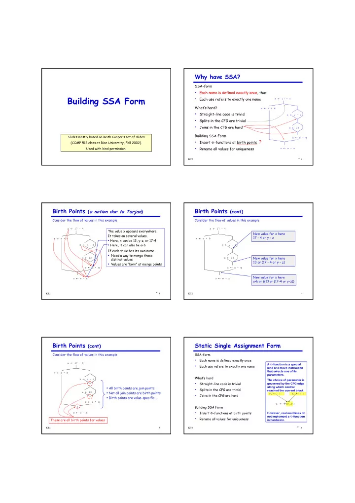
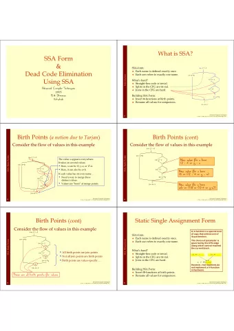
Why have SSA? SSA-form • Each name is defined exactly once, thus Building SSA Form • Each use refers to exactly one name x ← 17 - 4 What’s hard? x ← a + b • Straight-line code is trivial x ← y - z • Splits in the CFG are trivial • Joins in the CFG are hard x ← 13 Building SSA Form Slides mostly based on Keith Cooper’s set of slides z ← x * q ? • Insert Φ -functions at birth points (COMP 512 class at Rice University, Fall 2002). • Used with kind permission. Rename all values for uniqueness s ← w - x * KT2 2 Birth Points ( a notion due to Tarjan ) Birth Points (cont) Consider the flow of values in this example Consider the flow of values in this example x ← 17 - 4 x ← 17 - 4 The value x appears everywhere New value for x here It takes on several values. 17 - 4 or y - z x ← a + b x ← a + b • Here, x can be 13, y-z, or 17-4 • Here, it can also be a+b x ← y - z x ← y - z If each value has its own name … • Need a way to merge these x ← 13 x ← 13 New value for x here distinct values 13 or (17 - 4 or y - z) • Values are “born” at merge points z ← x * q z ← x * q New value for x here s ← w - x s ← w - x a+b or ((13 or (17-4 or y-z)) * KT2 3 KT2 4 Birth Points (cont) Static Single Assignment Form Consider the flow of values in this example SSA-form • Each name is defined exactly once x ← 17 - 4 A Φ -function is a special • Each use refers to exactly one name kind of a move instruction that selects one of its x ← a + b parameters. What’s hard x ← y - z The choice of parameter is • Straight-line code is trivial governed by the CFG edge • All birth points are join points along which control • Splits in the CFG are trivial reached the current block. x ← 13 • Not all join points are birth points y 1 ← ... y 2 ← ... • Joins in the CFG are hard • Birth points are value-specific … z ← x * q y 3 ← Φ (y 1 ,y 2 ) Building SSA Form • Insert Φ -functions at birth points s ← w - x However, real machines do not implement a Φ -function • Rename all values for uniqueness These are all birth points for values in hardware. * KT2 5 KT2 6

SSA Construction Algorithm (High-level sketch) SSA Construction Algorithm (Less high-level) 1. Insert Φ -functions 1. Insert Φ -functions at every join for every name 2. Rename values 2. Solve reaching definitions 3. Rename each use to the def that reaches it ( will be unique ) … that’s all ... … of course, there is some bookkeeping to be done ... * KT2 7 KT2 8 Reaching Definitions Domain is | DE ONS |, same SSA Construction Algorithm (Less high-level) DEFI FINI NITI TIONS as number of operations The equations 1. Insert Φ -functions at every join for every name R EACHES ( n 0 ) = Ø 2. Solve reaching definitions R EACHES ( n ) = ∪ p ∈ preds(n) D EF O UT ( p ) ∪ (R EACHES ( p ) ∩ S URVIVED ( p )) 3. Rename each use to the def that reaches it ( will be unique ) • R EACHES ( n ) is the set of definitions that reach block n Builds maximal SSA • D EF O UT ( n ) is the set of definitions in n that reach the end of n What’s wrong with this approach • S URVIVED ( n ) is the set of defs not obscured by a new def in n • Too many Φ -functions ( precision ) Computing R EACHES ( n ) • Too many Φ -functions ( space ) • Use any data-flow method ( i.e., the iterative method ) • Too many Φ -functions ( time ) • This particular problem has a very-fast solution ( Zadeck ) • Need to relate edges to Φ -functions parameters ( bookkeeping ) To do better, we need a more complex approach F.K. Zadeck, “Incremental data-flow analysis in a structured program editor,” Proceedings of the S IGPLAN 84 Conf. on Compiler Construction , June, 1984, pages 132-143. * KT2 9 KT2 10 SSA Construction Algorithm (Less high-level) SSA Construction Algorithm (Less high-level) 1. Insert Φ -functions 2. Rename variables in a pre-order walk over dominator tree (use an array of stacks, one stack per global name) a.) calculate dominance frontiers Moderately complex Staring with the root block, b 1 counter per name for subscripts b.) find global names for each name, build a list of blocks that define it a.) generate unique names for each Φ -function and push them on the appropriate stacks c.) insert Φ -functions Compute list of blocks where each name is assigned. Use this list as the worklist. b.) rewrite each operation in the block ∀ global name n i. Rewrite uses of global names with the current version ∀ block b in which n is defined This adds to (from the stack) ∀ block d in b ’s dominance frontier the worklist ! ii. Rewrite definition by inventing & pushing new name insert a Φ -function for n in d { Creates the iterated add d to n ’s list of defining blocks c.) fill in Φ -function parameters of successor blocks dominance frontier d.) recurse on b ’s children in the dominator tree Reset the state e.) < on exit from block b > pop names generated in b from stacks Use a checklist to avoid putting blocks on the worklist twice; keep another checklist to avoid inserting the same Φ -function twice. Need the end-of-block name for this path * * KT2 11 KT2 12

Aside on Terminology: Dominators Dominators (cont) Definitions Dominators have many uses in program analysis & transformation • x dominates y if and only if every path from the entry of the Finding loops A control-flow graph to the node for y includes x m 0 ← a + b • Building SSA form n 0 ← a + b • By definition, x dominates x • Making code motion decisions B C • We associate a Dom set with each node p 0 ← c + d q 0 ← a + b r 0 ← c + d r 1 ← c + d • |Dom( x )| ≥ 1 Dominator sets Dominator tree D E e 0 ← b + 18 e 1 ← a + 17 s 0 ← a + b t 0 ← c + d A u 0 ← e + f u 1 ← e + f Block Dom IDom A A – Immediate dominators B A,B A B C G F e 3 ← φ (e 0 ,e 1 ) • For any node x , there must be a y in Dom( x ) such that y is closest u 2 ← φ (u 0 ,u 1 ) C A,C A v 0 ← a + b to x D A,C,D C w 0 ← c + d D E F x 0 ← e + f E A,C,E C • We call this y the immediate dominator of x F A,C,F C G A,G A • As a matter of notation, we write this as IDom( x ) G r 2 ← φ (r 0 ,r 1 ) y 0 ← a + b • Let’s look at how to compute dominators… z 0 ← c + d By convention, IDom( x 0 ) is not defined for the entry node x 0 KT2 13 KT2 * 14 Example SSA Construction Algorithm (Low-level detail) Computing Dominance • Progress of iterative solution for D OM First step in Φ -function insertion computes dominance. B 0 • Iter- D OM ( n ) A node n dominates m iff n is on every path from n 0 to m. B 1 ation 0 1 2 3 4 5 6 7 Every node dominates itself 0 0 N N N N N N N > 1 0 0,1 0,1,2 0,1,3 0,1,3,4 0,1,3,5 0,1,3,6 0,1,7 n ’s immediate dominator is its closest dominator, ID OM ( n ) † > 2 0 0,1 0,1,2 0,1,3 0,1,3,4 0,1,3,5 0,1,3,6 0,1,7 B 2 B 3 D OM ( n 0 ) = { n 0 } Initially, D OM (n) = N, Results of iterative solution for D OM ∀ n ≠ n 0 B 4 B 5 D OM ( n ) = { n } ∪ ( ∩ p ∈ preds(n) D OM ( p )) 0 1 2 3 4 5 6 7 D OM 0 0,1 0,1,2 0,1,3 0,1,3,4 0,1,3,5 0,1,3,6 0,1,7 B 6 ID OM 0 1 1 3 3 3 1 Computing DOM • B 7 These equations form a rapid data-flow framework. • Iterative algorithm will solve them in d(G) + 3 passes Flow Graph Each pass does N unions & E intersections, > E is O( N 2 ) ⇒ O( N 2 ) work > † ID OM (n ) ≠ n , unless n is n 0 , by KT2 15 KT2 * 16 convention. Example Example Progress of iterative solution for D OM B 0 B 0 Dominance Frontiers & Φ -Function Insertion Iter- D OM ( n ) • A definition at n forces a Φ -function at m iff B 1 x ← Φ (...) B 1 ation 0 1 2 3 4 5 6 7 n ∉ D OM ( m ) but n ∈ D OM (p) for some p ∈ preds(m) 0 0 N N N N N N N 1 0 0,1 0,1,2 0,1,3 0,1,3,4 0,1,3,5 0,1,3,6 0,1,7 • DF( n ) is fringe just beyond region n dominates 2 0 0,1 0,1,2 0,1,3 0,1,3,4 0,1,3,5 0,1,3,6 0,1,7 B 2 B 3 B 2 B 3 0 1 2 3 4 5 6 7 Results of iterative solution for D OM D OM 0 0,1 0,1,2 0,1,3 0,1,3,4 0,1,3,5 0,1,3,6 0,1,7 x ← ... B 4 B 5 B 4 B 5 DF – – 7 7 6 6 7 1 0 1 2 3 4 5 6 7 D OM 0 0,1 0,1,2 0,1,3 0,1,3,4 0,1,3,5 0,1,3,6 0,1,7 B 6 x ← Φ (...) B 6 ID OM 0 1 1 3 3 3 1 • DF(4) is {6}, so ← in 4 forces a Φ -function in 6 x ← Φ (...) B 7 B 7 • ← in 6 forces a Φ -function in DF(6) = {7} • ← in 7 forces a Φ -function in DF(7) = {1} There are asymptotically faster algorithms. Dominance Dominance • ← in 1 forces a Φ -function in DF(1) = Ø ( halt ) Tree Frontiers With the right data structures, the iterative algorithm can be made faster. For each assignment, we insert the Φ -functions See Cooper, Harvey, and Kennedy. * KT2 17 KT2 18