Brownian Motion Area with Generatingfunctionology Uwe Schwerdtfeger - PowerPoint PPT Presentation
Introduction and Results Proofs Applications Brownian Motion Area with Generatingfunctionology Uwe Schwerdtfeger RMIT University/University of Melbourne Alexander von Humboldt Foundation Monash University 3 August, 2011 U. Schwerdtfeger
Introduction and Results Proofs Applications Brownian Motion Area with Generatingfunctionology Uwe Schwerdtfeger RMIT University/University of Melbourne Alexander von Humboldt Foundation Monash University 3 August, 2011 U. Schwerdtfeger Brownian Motion Area
Introduction and Results Proofs Applications Some continuous time processes... A Brownian Motion of duration 1 is a stochastic process B ( t ) , t ∈ [0 , 1] such that ◮ t �→ B ( t ) is a.s. continuous, B (0) = 0 , ◮ for s < t , B ( t ) − B ( s ) ∼ N (0 , t − s ) and ◮ increments are independent. A Brownian Meander M ( t ) , t ∈ [0 , 1] is a BM B ( t ) conditioned on B ( s ) ≥ 0 , s ∈ ]0 , 1] . A Brownian Excursion E ( t ) , t ∈ [0 , 1] is M ( t ) conditioned on M (1) = 0 (quick and dirty def.). U. Schwerdtfeger Brownian Motion Area
Introduction and Results Proofs Applications ... and their discrete counterparts The Bernoulli Random Walk B n ( k ) on Z , k ∈ { 0 , 1 , . . . , n } , with ◮ B n (0) = 0 , ◮ B n ( k + 1) − B n ( k ) ∈ {− 1 , 1 } , each with prob. 1 / 2 . The Bernoulli Meander M n ( k ) , k ∈ { 0 , . . . , n } on Z ≥ 0 is B n ( k ) conditioned to stay non-negative. The Bernoulli Excursion E 2 n ( k ) , k ∈ { 0 , . . . , 2 n } on Z ≥ 0 is M 2 n ( k ) conditioned on M 2 n (2 n ) = 0 . U. Schwerdtfeger Brownian Motion Area
Introduction and Results Proofs Applications Scaling limits For n − → ∞ we have the weak limits � � 1 √ n B n ( ⌊ nt ⌋ ) , t ∈ [0 , 1] − → {B ( t ) , t ∈ [0 , 1] } , ◮ � � 1 √ n M n ( ⌊ nt ⌋ ) , t ∈ [0 , 1] − → {M ( t ) , t ∈ [0 , 1] } , ◮ � � 1 2 n E 2 n ( ⌊ 2 nt ⌋ ) , t ∈ [0 , 1] − → {E ( t ) , t ∈ [0 , 1] } . ◮ √ U. Schwerdtfeger Brownian Motion Area
Introduction and Results Proofs Applications Drmota (2003): Weak limits imply moment convergence for certain functionals. E.g. for area (i.e. integrals) ��� 1 � r � 1 → E [ EA r ] , √ E 2 n ( ⌊ 2 nt ⌋ ) dt − E 2 n 0 ��� 1 � r � 1 → E [ MA r ] , √ n M n ( ⌊ nt ⌋ ) dt − E 0 for n − → ∞ , where � 1 � 1 EA := E ( t ) dt , MA := M ( t ) dt . 0 0 So studying functionals on E or M amounts to studying the discrete models! U. Schwerdtfeger Brownian Motion Area
Introduction and Results Proofs Applications Particularly EA appears in a number of discrete contexts, e.g. ◮ Construction costs of hash tables, ◮ cost of breadth first search traversal of a random tree, ◮ path lengths in random trees, ◮ area of polyominoes, ◮ enumeration of connected graphs. Many of the discrete results rely on recursions for the moments of EA and MA found by Tak´ acs (1991,1995) studying E 2 n and M n . U. Schwerdtfeger Brownian Motion Area
Introduction and Results Proofs Applications Results We choose a different combinatorial approach and obtain ◮ new formulae for E ( EA r ) and E ( MA r ) , ◮ the joint distribution of ( MA , M (1)) in terms of the joint moments E ( MA r M (1) s ) , ◮ the joint distribution of (signed) areas and endpoint of B , and as an application of these ◮ area of discrete meanders with arbitrary finite step sets, ◮ area distribution of column convex polyominoes. U. Schwerdtfeger Brownian Motion Area
Introduction and Results Proofs Applications In the discrete world, we can write the joint distribution of the random variables n � M n ( k ) and H n = M n ( n ) A n = k =0 as p n , k , l P ( A n = k , H n = l ) = , � r , s p n , r , s where p n , k , l is the number of meanders of length n , area k and final height l . U. Schwerdtfeger Brownian Motion Area
Introduction and Results Proofs Applications The generating function of the class of meanders is the formal power series � � p n , k , l q k u l z n , M ( z , q , u ) = n k , l The above probabilities can be rewritten as p n , k , l P ( A n = k , H n = l ) = � r , s p n , r , s � z n q k u l � M ( z , q , u ) = . [ z n ] M ( z , 1 , 1) U. Schwerdtfeger Brownian Motion Area
Introduction and Results Proofs Applications � � p n , k , l q k u l z n , M ( z , q , u ) = n k , l and � z n q k u l � M ( z , q , u ) P ( A n = k , H n = l ) = . [ z n ] M ( z , 1 , 1) With this representation the moments take a particularly nice form: � E ( A r n H s k r l s P ( A n = k , H n = l ) n ) = k , l � r � � s M ( z , 1 , 1) � [ z n ] q ∂ u ∂ ∂ q ∂ u = . [ z n ] M ( z , 1 , 1) So: large n behaviour of the moments by coefficient asymptotics of the above series. U. Schwerdtfeger Brownian Motion Area
Introduction and Results Proofs Applications Singularity analysis (Flajolet, Odlyzko 1990) Transfer Theorem: Let F ( z ) = � f n z n be analytic in an indented disk and F ( z ) ∼ (1 − µ z ) − α ( z − → 1 /µ ) . Then 1 f n ∼ [ z n ] (1 − µ z ) − α ∼ Γ( α ) × n α − 1 × µ n ( n − → ∞ ) . For example, it turns out, that � ∂ � r � ∂ � s b r , s M ( z , 1 , 1) ∼ ( z − → 1 / 2) , ∂ q ∂ u (1 − 2 z ) 3 r / 2+ s / 2+1 / 2 U. Schwerdtfeger Brownian Motion Area
Introduction and Results Proofs Applications Functional equation for M ( z , q , u ) . The recursive description of the set of meanders { meanders of length n } ≃ { meanders of length n − 1 } × {ր , ց} \ { excursions of length n − 1 } × {ց} translates into � zuq + z � − E ( z , q ) z M ( z , q , u ) = 1 + M ( z , q , uq ) uq , uq E ( z , q ) is the generating function of excursions. U. Schwerdtfeger Brownian Motion Area
Introduction and Results Proofs Applications Solution to the equation for q = 1 by the kernel method: − z ( u − u 1 ( z ))( u − v 1 ( z )) M ( z , 1 , u ) = u − zE ( z , 1) . √ √ 1 − 4 z 2 1 − 4 z 2 where u 1 ( z ) = 1 − and v 1 ( z ) = 1+ . 2 z 2 z Substitution of u = u 1 ( z ) yields √ 1 − 4 z 2 E ( z , 1) = u 1 ( z ) = 1 − , 2 z 2 z and finally 1 M ( z , 1 , u ) = − z ( u − v 1 ( z )) . U. Schwerdtfeger Brownian Motion Area
Introduction and Results Proofs Applications � r � ∂ � s M ( z , 1 , u ) can in principle be � ∂ The partial derivatives ∂ q ∂ u obtained inductively by taking derivatives of the functional equation (and setting q = 1). ◮ Each derivative w.r.t. u produces one new unknown function � r � ∂ � s +1 M ( z , 1 , u ) . � ∂ ∂ q ∂ u ◮ Each derivative w.r.t. q produces two new unknowns, � r +1 � r +1 � ∂ � s M ( z , 1 , u ) and hence � � ∂ ∂ E ( z , 1) and ∂ q ∂ q ∂ u requires another application of the kernel method. U. Schwerdtfeger Brownian Motion Area
Introduction and Results Proofs Applications � r � ∂ � s M ( z , 1 , u ) and for � ∂ The exact expressions for ∂ q ∂ u � r � � s M ( z , 1 , 1) � q ∂ u ∂ [ z n ] ∂ q ∂ u E ( A r n H s n ) = . [ z n ] M ( z , 1 , 1) are getting intractable. But we can keep track of the singular behaviour of � r � ∂ � r � ∂ � s M ( z , 1 , 1) and � s M ( z , 1 , u 1 ( z )) and via � � ∂ ∂ ∂ q ∂ u ∂ q ∂ u singularity analysis large n asymptotics for the moments. U. Schwerdtfeger Brownian Motion Area
Introduction and Results Proofs Applications One proceeds in two steps: First show by induction � ∂ � r � ∂ � s a r , s M ( z , 1 , u 1 ( z )) ∼ ( z − → 1 / 2) , (1 − 2 z ) 3 r / 2+ s / 2+1 / 2 ∂ q ∂ u where a r , s = a r , s − 1 + ( s + 2) a r − 1 , s +2 , and then by induction � ∂ � r � ∂ � s b r , s M ( z , 1 , 1) ∼ ( z − → 1 / 2) , (1 − 2 z ) 3 r / 2+ s / 2+1 / 2 ∂ q ∂ u where b r , s = b r , s − 2 + ( s + 1) b r − 1 , s +1 , ( s ≥ 1) , b r , 0 = b r − 1 , 1 + a r − 1 , 1 . U. Schwerdtfeger Brownian Motion Area
Introduction and Results Proofs Applications Application of the transfer theorem finally yields: Γ(1 / 2) n ) ∼ b r , s Γ((3 r + s ) / 2) n (3 r + s ) / 2 , E ( A r n H s b 0 , 0 and hence (after rescaling n − 3 / 2 A n and n − 1 / 2 H n ) ◮ b r , s is essentially E ( MA r M (1) s ) , ◮ similarly a r − 1 , 1 is essentially E ( EA r ) . U. Schwerdtfeger Brownian Motion Area
Introduction and Results Proofs Applications Discrete meanders and excursions with arbitrary finite step sets: No result on convergence to M resp. E ! But: ◮ Generating function satisfies a similar functional equation. ◮ Area moments for meanders and excursions can be computed in the same fashion, ◮ and are expressed in terms of the very same b r , s resp. a r − 1 , 1 ! Result depends on the sign of the drift = mean of the step set. U. Schwerdtfeger Brownian Motion Area
Introduction and Results Proofs Applications Column convex polyominoes: Area distribution on polyominoes with fixed perimeter n . ◮ Similar functional equation as above. ◮ Similar arguments yield an EA limit law as n − → ∞ . U. Schwerdtfeger Brownian Motion Area
Introduction and Results Proofs Applications Acknowledgement Thank you for your attention! And thanks to ◮ Alexander von Humboldt Foundation ◮ RMIT University ◮ The ARC Centre of Excellence Mathematics and Statistics of Complex Systems (MASCOS) for financial support. U. Schwerdtfeger Brownian Motion Area
Recommend
More recommend
Explore More Topics
Stay informed with curated content and fresh updates.
