Branch Flow Model relaxations, convexification Masoud Farivar - PowerPoint PPT Presentation
Branch Flow Model relaxations, convexification Masoud Farivar Steven Low Computing + Math Sciences Electrical Engineering Caltech May 2012 Motivations Global trends 1 Proliferation renewables ! Driven by sustainability ! Enabled by
Branch Flow Model relaxations, convexification Masoud Farivar Steven Low Computing + Math Sciences Electrical Engineering Caltech May 2012
Motivations
Global trends 1 Proliferation renewables ! Driven by sustainability ! Enabled by policy and investment
Sustainability challenge Electricity generation 1971-2007 2007: 19,800 TWh 1973: 6,100 TWh In 2009, 1.5B people US CO 2 emission have no electricity Elect generation: 40% Sources: International Energy Agency, 2009 Transportation: 20% DoE, Smart Grid Intro, 2008
Worldwide energy demand: 16 TW Wind power over land (exc. Antartica) electricity demand: 70 – 170 TW 2.2 TW wind capacity (2009) : 159 GW grid-tied PV capacity (2009) : 21 GW Source: Renewable Energy Global Status Report, 2010 Solar power over land Source: M. Jacobson, 2011 340 TW
Uncertainty High Levels of Wind and Solar PV Will Present an Operating Challenge! Source: Rosa Yang, EPRI
Global trends 1 Proliferation of renewables ! Driven by sustainability ! Enabled by policy and investment 2 Migration to distributed arch ! 2-3x generation efficiency ! Relief demand on grid capacity
Large active network of DER DER: PVs, wind turbines, batteries, EVs, DR loads
Large active network of DER Millions of active endpoints introducing rapid large � random fluctuations � in supply and demand � DER: PVs, wind turbines, EVs, batteries, DR loads
Implications Current control paradigm works well today ! Low uncertainty, few active assets to control ! Centralized, open-loop, human-in-loop, worst-case preventive ! Schedule supplies to match loads Future needs ! Fast computation to cope with rapid, random, large fluctuations in supply, demand, voltage, freq ! Simple algorithms to scale to large networks of active DER ! Real-time data for adaptive control, e.g. real-time DR
Key challenges Nonconvexity ! Convex relaxations Large scale ! Distributed algorithms Uncertainty ! Risk-limiting approach
Optimal power flow (OPF) OPF is solved routinely to determine ! How much power to generate where ! Market operation & pricing ! Parameter setting, e.g. taps, VARs Non-convex and hard to solve ! Huge literature since 1962 ! Common practice: DC power flow (LP)
Optimal power flow (OPF) Problem formulation Carpentier 1962 ! Computational techniques Dommel & Tinney 1968 ! Surveys: Huneault et al 1991, Momoh et al 2001, ! Pandya et al 2008 Bus injection model: SDP relaxation Bai et al 2008, 2009, Lavaei et al 2010, 2012 ! Bose et al 2011, Zhang et al 2011, Sojoudi et al 2012 ! Lesieutre et al 2011 ! Branch flow model: SOCP relaxation Baran & Wu 1989, Chiang & Baran 1990, Taylor 2011, ! Farivar et al 2011
Application: Volt/VAR control Motivation ! Static capacitor control cannot cope with rapid random fluctuations of PVs on distr circuits Inverter control ! Much faster & more frequent ! IEEE 1547 does not optimize VAR currently (unity PF)
!"#$%#&$%'"(#)%*#)+#,"&% c p i g p i -./+)+0#(%$+12)+34,"&%% "5%6("#$7%1"(#)8%5")%9#(#3#1:%
'4..#);% • <")=%)=(+#3(=%"/=)#,"&% • -&=)>;%1#?+&>1%
Outline Branch flow model and OPF Solution strategy: two relaxations ! Angle relaxation ! SOCP relaxation Convexification for mesh networks Extension
Two models g c s j s j k j i S jk 3)#&0:% S ij @"A% ! ! S j = S jk k 341%% +&B=0,"&%
Two models j i k z ij V i V j I ij branch ! ! current I j = I jk k bus current
Two models S i = V i ! ! * I i V i V j * S ij = V i I ij Equivalent models of Kirchhoff laws ! Bus injection model focuses on nodal vars ! Branch flow model focuses on branch vars
Two models S i = V i ! ! * I i V i V j * S ij = V i I ij 1. What is the model? 2. What is OPF in the model? 3. What is the solution strategy?
let’s start with something familiar
Bus injection model ! S j = V j ! * for all j I j power definition ! I = YV Kirchhoff law ! S j = ! s j for all j power balance admittance matrix: S j = V j ! ! * I j # ! y ik if i = j c ! s j g s j = s j % k ~ i % Y ij : = " y ij if i ~ j $ % 0 else % &
Bus injection model ! S j = V j ! * for all j I j power definition ! I = YV Kirchhoff law ! S j = ! s j for all j power balance x : = ! S , ! ) , s : = s c ! s g ( variables ! I , V , s
Bus injection model: OPF f j Re ! ( ) ( ) ! min S j e.g. generation cost j x : = ! S , ! over ! ( ) I , V , s subject to ! I = YV Kirchhoff law ! S j = " s j ! S j = V j ! power balance * I j s j # s j # s j V k # | V k | # V k
Bus injection model: OPF In terms of V : " * * min tr M k VV P k = tr ! k VV k ! G * Q k = tr " k VV over V g # P g # P d $ tr % k VV * $ P k d s.t. P k * + Y k k k # & ! k := Y k g # Q k g # Q k d $ tr & k VV % ( * $ Q k d Q k 2 $ ' * ) Y k 2 2 $ tr J k VV # & * $ V k V k " k := Y k % ( 2 i $ ' Key observation [Bai et al 2008] : OPF = rank constrained SDP
Bus injection model: OPF " min tr M k W k ! G over W positive semidefinite matrix s.t. P k # tr $ k W # P k Q k # tr % k W # Q k 2 2 # tr J k W # V k V k W & 0, rank W = 1 convex relaxation: SDP
Bus injection model: SDR Non-convex QCQP Rank-constrained SDP Relax the rank constraint and solve the SDP Bai 2008 Does the optimal solution satisfy the rank-constraint? yes no We are done! Solution may not be meaningful Lavaei 2010, 2012 Radial: Bose 2011, Zhang 2011 Lesiertre 2011 Sojoudi 2011
Bus injection model: summary OPF = rank constrained SDP Sufficient conditions for SDR to be exact ! Mesh: must solve SDR to check ! Tree: depends only on constraint pattern
Two models S i = V i ! ! * I i V i V j * S ij = V i I ij 1. What is the model? 2. What is OPF in the model? 3. What is the solution strategy?
Branch flow model * for all i ! j S ij = V i I ij power def V i ! V j = z ij I ij for all i " j Ohm’s law ( ) 2 # # S ij ! z ij I ij S jk = s j for all j power balance ! i " j j " k sending sending end pwr loss end pwr s j
Branch flow model * for all i ! j S ij = V i I ij power def V i ! V j = z ij I ij for all i " j Ohm’s law ( ) 2 # # S ij ! z ij I ij S jk = s j for all j power balance ! i " j j " k ) , s : = s c ! s g ( variables x : = S , I , V , s branch flows
Branch flow model * for all i ! j S ij = V i I ij power def V i ! V j = z ij I ij for all i " j Ohm’s law ( ) 2 # # S ij ! z ij I ij S jk = s j for all j power balance ! i " j j " k ) , s : = s c ! s g ( variables x : = S , I , V , s y : = h ( x ): = S , ! , v , s projection ˆ ( )
Branch flow model: OPF 2 + 2 ! ! min r I ij V i ! i ij i ~ j i over ( S , I , V , s g , s c ) 9*H%60"&1=)?#,"&% )=#(%/"A=)%("11% g " s i g " s i g s i " s i c s. t. s i ?"(2#>=%)=$40,"&8%% v i " v i " v i 2 + s j c " s j C+)0:"DE1%!#AF% ! g S ij = S jk + z ij I ij k : j ~ k G:.E1%!#AF% * S ij = V i I ij V j = V i ! z ij I ij
Branch flow model: OPF ( ) min f h ( x ) over x : = ( S , I , V , s g , s c ) g ! s i g ! s i g s i ! s i c s. t. s i 2 ! v i $=.#&$% v i ! V i )=1/"&1=% ( ) c ! s j 2 # # g S ij ! z ij I ij S jk = s j ! 3)#&0:%@"A% i " j j " k ."$=(% * S ij = V i I ij V j = V i ! z ij I ij
Branch flow model: OPF ( ) min f h ( x ) over x : = ( S , I , V , s g , s c ) g ! s i g ! s i g s i ! s i c s. t. s i 2 ! v i >=&=)#,"&7% v i ! V i *IH%0"&2)"(% ( ) c ! s j 2 # # g S ij ! z ij I ij S jk = s j ! 3)#&0:%@"A% i " j j " k ."$=(% * S ij = V i I ij V j = V i ! z ij I ij
Outline Branch flow model and OPF Solution strategy: two relaxations ! Angle relaxation ! SOCP relaxation Convexification for mesh networks Extension
Solution strategy OPF nonconvex inverse angle projection relaxation for tree OPF-ar nonconvex conic exact relaxation relaxation OPF-cr convex
Angle relaxation ( ) c ! s j 2 # # g S ij ! z ij I ij S jk = s j ! 3)#&0:%@"A% i " j j " k ."$=(% * S ij = V i I ij V j = V i ! z ij I ij
Angle relaxation ( ) c ! s j 2 # # g S ij ! z ij I ij S jk = s j ! 3)#&0:%@"A% i " j j " k ."$=(% * S ij = V i I ij V j = V i ! z ij I ij eliminate angles 2 I ij 2 + 2 Re z ij 2 = V j 2 ( ) ! z ij * S ij V i /"+&21%)=(#J=$%% 2"%0+)0(=1%K% 2 2 = S ij I ij 2 V i
Angle relaxation ( ) c ! s j 2 # # g S ij ! z ij I ij S jk = s j ! ( ) S , I , V , s i " j j " k * S ij = V i I ij V j = V i ! z ij I ij 2 I ij 2 + 2 Re z ij 2 = V j 2 ( ) ! z ij * S ij V i 2 2 = S ij I ij 2 V i
Angle relaxation ( ) c ! s j 2 # # g S ij ! z ij I ij S jk = s j ! ( ) S , I , V , s i " j j " k * S ij = V i I ij V j = V i ! z ij I ij 2 I ij 2 + 2 Re z ij 2 = V j 2 ( ) ! z ij * S ij V i 2 2 = S ij 2 ! ij : = I ij S , ! , v , s I ij ( ) 2 V i 2 v i : = V i
Recommend
More recommend
Explore More Topics
Stay informed with curated content and fresh updates.
