Bootstrapping Statistical Parsers from Small Datasets Anoop Sarkar - PowerPoint PPT Presentation

Bootstrapping Statistical Parsers from Small Datasets Anoop Sarkar Department of Computing Science Simon Fraser University anoop@cs.sfu.ca http://www.cs.sfu.ca/˜anoop 1

Overview • Task: find the most likely parse for natural language sentences • Approach: rank alternative parses with statistical methods trained on data annotated by experts (labelled data) • Focus of this talk: 1. Machine learning by combining different methods in parsing: PCFG and Tree-adjoining grammar 2. Weakly supervised learning: combine labelled data with unlabelled data to improve performance in parsing using co-training 2

A Key Problem in Processing Language: Ambiguity: (Church and Patil 1982; Collins 1999) • Part of Speech ambiguity saw → noun saw → verb • Structural ambiguity: Prepositional Phrases I saw (the man) with the telescope I saw (the man with the telescope) • Structural ambiguity: Coordination a program to promote safety in ((trucks) and (minivans)) a program to promote ((safety in trucks) and (minivans)) ((a program to promote safety in trucks) and (minivans)) 3

Ambiguity ← attachment choice in alternative parses NP NP NP VP NP VP a program to VP a program to VP promote NP promote NP NP PP NP and NP safety in NP safety PP minivans trucks and minivans in trucks 4

Parsing as a machine learning problem • S = a sentence T = a parse tree A statistical parsing model defines P ( T | S ) • Find best parse: arg max P ( T | S ) T • P ( T | S ) = P ( T , S ) P ( S ) = P ( T , S ) • Best parse: arg max P ( T , S ) T • e.g. for PCFGs: P ( T , S ) = � i = 1 ... n P (RHS i | LHS i ) 5

Parsing as a machine learning problem • Training data: the Penn WSJ Treebank (Marcus et al. 1993) • Learn probabilistic grammar from training data • Evaluate accuracy on test data • A standard evaluation: Train on 40,000 sentences Test on 2,300 sentences • The simplest technique: PCFGs perform badly Reason: not sensitive to the words 6

Machine Learning for ambiguity resolution: prepositional phrases • What is right analysis for: Calvin saw the car on the hill with the telescope • Compare with: Calvin bought the car with anti-lock brakes and Calvin bought the car with a loan • (bought, with, brakes) and (bought, with, loan) are useful features to solve this apparently AI-complete problem 7

Method Accuracy Always noun attachment 59.0 Most likely for each preposition 72.2 Average Human (4 head words only) 88.2 Average Human (whole sentence) 93.2 Lexicalized Model (Collins and Brooks 1995) 84.5 Lexicalized Model + Wordnet (Stetina and Nagao 1998) 88.0 8

Statistical Parsing the company ’s clinical trials of both its animal and human-based insulins indicated no difference in the level of hypoglycemia between users of either product S( indicated ) NP( trials ) VP( indicated ) the company ’s clinical trials . . . V( indicated ) NP( di ff erence ) PP( in ) indicated no di ff erence P( in ) NP( level ) in the level of . . . Use a probabilistic lexicalized grammar from the Penn WSJ Treebank for parsing . . . 9

Bilexical CFG (Collins-CFG): dependencies between pairs of words • Full context-free rule: VP( indicated ) → V-hd( indicated ) NP( difference ) PP( in ) • Each rule is generated in three steps (Collins 1999) : 1. Generate head daughter of LHS: VP( indicated ) → V-hd( indicated ) 2. Generate non-terminals to left of head daughter:  . . . V-hd( indicated ) 10

3. Generate non-terminals to right of head daughter: – V-hd( indicated ) . . . NP( difference ) – V-hd( indicated ) . . . PP( in ) – V-hd( indicated ) . . . 

Lexicalized Tree Adjoining Grammars (LTAG): Different Modeling of Bilexical Dependencies NP NP NP ∗ SBAR VP the store WH ↓ S VP ∗ NP WH NP ↓ VP last week which NP bought NP IBM ǫ 11

Performance of supervised statistical parsers ≤ 40 wds ≤ 40 wds ≤ 100 wds ≤ 100 wds System LP LR LP LR PCFG (Collins 99) 88.5 88.7 88.1 88.3 LTAG (Sarkar 01) 88.63 88.59 87.72 87.66 LTAG (Chiang 00) 87.7 87.7 86.9 87.0 PCFG (Charniak 99) 90.1 90.1 89.6 89.5 Re-ranking (Collins 00) 90.1 90.4 89.6 89.9 • Labelled Precision = number of correct constituents in proposed parse number of constituents in proposed parse • Labelled Recall = number of correct constituents in proposed parse number of constituents in treebank parse 12

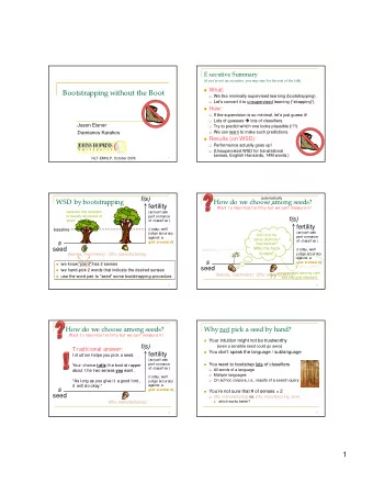
Bootstrapping • Current state-of-the-art in parsing on the Penn WSJ Treebank dataset is approx 90% accuracy • However this accuracy is obtained with 1M words of human annotated data (40K sentences) • Exploring methods that can exploit unlabelled data is an important goal: – What about different languages? The Penn Treebank took several years with many linguistic experts and millions of dollars to produce. Unlikely to happen for all other languages of interest. 13

– What about different genres? Porting a parser trained on newspaper text and using it on fiction is a challenge. – Combining labelled and unlabelled data is an interesting challenge for machine learning. • In this talk, we will consider bootstrapping using unlabelled data. • Bootstrapping refers to a problem setting in which one is given a small set of labelled data and a large set of unlabelled data, and the task is to extract new labelled instances from the unlabelled data. • The noise introduced by the new automatically labelled instances has to be offset by the utility of training on those instances.

Multiple Learners and the Bootstrapping problem • With a single learner, the simplest method of bootstrapping is called self-training . • The high precision output of a classifier can be treated as new labelled instances (Yarowsky, 1995). • With multiple learners, we can exploit the fact that they might: – Pay attention to different features in the labelled data. – Be confident about different examples in the unlabelled data. – Combine multiple learners using the co-training algorithm. 14

Co-training • Pick two “views” of a classification problem. • Build separate models for each of these “views” and train each model on a small set of labelled data. • Sample an unlabelled data set and to find examples that each model independently labels with high confidence. • Pick confidently labelled examples and add to labelled data. Iterate. • Each model labels examples for the other in each iteration. 15

An Example: (Blum and Mitchell 1998) • Task: Build a classifier that categorizes web pages into two classes, + : is a course web page , − : is not a course web page • Usual model: build a Naive Bayes model: P ( c k ) × P ( x | c k ) P [ C = c k | X = x ] = P ( x ) � P ( x | c k ) = P ( x j | c k ) x j ∈ x 16

• Each labelled example has two views: x 1 Text in hyperlink: <a href=" . . . "> CSE 120, Fall semester </a> x 2 Text in web page: <html> . . . Assignment #1 . . . </html> • Documents in the unlabelled data where C = c k is predicted with high confidence by classifier trained on view x 1 can be used as new training data for view x 2 and vice versa • Each view can be used to create new labelled data for the other view. • Combining labelled and unlabelled data in this manner outperforms using only the labelled data.

Theory behind co-training: (Abney, 2002) • For each instance x , we have two views X 1 ( x ) = x 1 , X 2 ( x ) = x 2 . x 1 , x 2 satisfy view independence if: Pr [ X 1 = x 1 | X 2 = x 2 , Y = y ] Pr [ X 1 = x 1 | Y = y ] = Pr [ X 2 = x 2 | X 1 = x 1 , Y = y ] Pr [ X 2 = x 2 | Y = y ] = • If H 1 , H 2 are rules that use only X 1 , X 2 respectively, then rule independence is: Pr [ F = u | G = v , Y = y ] = Pr [ F = u | Y = y ] where F ∈ H 1 and G ∈ H 2 (note that view independence implies rule independence) 17

Theory behind co-training: (Abney, 2002) • Deviation from conditional independence: d y = 1 � | Pr [ G = v | Y = y , F = u ] − Pr [ G = v | Y = y ] | 2 u , v • For all F ∈ H 1 , G ∈ H 2 such that q 1 − p 1 d y ≤ p 2 2 p 1 q 1 and min u Pr [ F = u ] > Pr [ F � G ] then Pr [ F � Y ] ≤ Pr [ F � G ] Pr [ ¯ ≤ F � Y ] Pr [ F � G ] we can choose between F and ¯ F using seed labelled data 18

Theory behind co-training: Pr [ F � Y ] ≤ Pr [ F � G ] G − + q p 2 2 + q 1 F − p 1 Positive Correlation, Y = + 19

Theory behind co-training • (Blum and Mitchell, 1998) prove that, when the two views are conditionally independent given the label, and each view is sufficient for learning the task, co-training can improve an initial weak learner using unlabelled data. • (Dasgupta et al, 2002) show that maximising the agreement over the unlabelled data between two learners leads to few generalisation errors (same independence assumption). • (Abney, 2002) argues that the independence assumption is extremely restrictive and typically violated in the data. He proposes a weaker independence assumption and a greedy algorithm that maximises agreement on unlabelled data. 20