12/20/2017 Lectures on Signals & systems Engineering Designed - PDF document
12/20/2017 Lectures on Signals & systems Engineering Designed and Presented by Dr. Ayman Elshenawy Elsefy Dept. of Systems & Computer Eng. Al-Azhar University Email : eaymanelshenawy@yahoo.com Chapter 9 Laplace Transform Applications
12/20/2017 Lectures on Signals & systems Engineering Designed and Presented by Dr. Ayman Elshenawy Elsefy Dept. of Systems & Computer Eng. Al-Azhar University Email : eaymanelshenawy@yahoo.com Chapter 9 Laplace Transform Applications 2 Chapter 9 The Laplace Transform Chapter 9 The Laplace Transform 𝒚 𝒖 = 𝒇 −𝒃𝒖 𝒗 𝒖 , 𝒃 > 𝟏, 𝒃 ∈ 𝑺 +∞ 𝒀 𝑻 = 𝒚 𝒖 𝒇 −𝒕𝒖 𝒆𝒖 −∞ +∞ +∞ 𝒇 −𝒃𝒖 𝒇 −𝒕𝒖 𝒆𝒖 𝒇 −𝒃𝒖 𝒗 𝒖 𝒇 −𝒕𝒖 𝒆𝒖 = = −∞ 𝟏 +∞ 𝒇 −(𝒕+𝒃)𝒖 𝒆𝒖 = −𝟐 𝒕 + 𝒃 𝒇 − 𝒕+𝒃 ∗∞ − 𝒇 − 𝒕+𝒃 ∗𝟏 = 𝟏 = −𝟐 𝟐 𝒕 + 𝒃 𝟏 − 𝟐 = 𝒕 + 𝒃 , 𝑺𝒇 𝒕 > −𝒃 1
12/20/2017 Chapter 9 The Laplace Transform Chapter 9 The Laplace Transform 𝒚 𝒖 = 𝒇 −𝒃𝒖 𝒗 −𝒖 , 𝒃 > 𝟏 +∞ 𝒚 𝒖 𝒇 −𝒕𝒖 𝒆𝒖 𝒀 𝑻 = −∞ +∞ 𝒇 −𝒃𝒖 𝒗 −𝒖 𝒇 −𝒕𝒖 𝒆𝒖 = −∞ 𝟏 𝟏 𝒇 −𝒃𝒖 𝒇 −𝒕𝒖 𝒆𝒖 = 𝒇 −(𝒕+𝒃)𝒖 𝒆𝒖 = −∞ −∞ = −𝟐 𝒕 + 𝒃 𝒇 − 𝒕+𝒃 ∗𝟏 − 𝒇 − 𝒕+𝒃 ∗−∞ = −𝟐 𝒕 + 𝒃 𝟐 − 𝟏 = −𝟐 𝒕 + 𝒃 , 𝑺𝒇 𝒕 < −𝒃 Chapter 9 The Laplace Transform Chapter 9 The Laplace Transform 2
12/20/2017 Zeroes and Poles of rational Laplace transform Zeroes and Poles of rational Laplace transform 𝑶(𝒕 ) 𝒀 𝒕 = 𝑬(𝒕 ) Zeroes of the Laplace transform N(s) = 0 If 𝒜 𝟐 is a zero, then 𝐘 𝒜 𝟐 = 𝟏 Poles of the Laplace transform D(s) = 0 𝒒 𝟐 = 𝟏 then 𝐘 𝒒 𝟐 = ∞ Region of Convergence ROC Region of Convergence ROC 3
12/20/2017 Region of Convergence ROC Chapter 9 The Laplace Transform Basic Laplace Pairs Poles ROC x t X s t 1 none Re s 1 s 0 u t Re s 0 s 1 u 0 t s Re s 0 s 1 s a e at Re u t s a s a 1 e at s a u t Re s a s a 14 Chapter 9 The Laplace Transform Chapter 9 The Laplace Transform j Example 9.13 L 1 Re s 1. t 1 X s Re s 1 1 s 1 1 1 0 L 2. u t Re s s j 1 X s Re s 1 0 2 1 s 1 s 2 L u t Re s s 2 1 1 X s X s X s 1 L 1 2 3. at e u t s 2 Re s a j s a Re s 2 1 at L e u t Re s a 2 s a 2 t x t e u t 15 16 4
12/20/2017 Chapter 9 The Laplace Transform Chapter 9 The Laplace Transform § 9.5.2 Time Shifting § 9.5.3 Shifting in s-Domain L Roc L Roc x t X s R x t X s R s t L Roc x t e X s s Roc R Re s L st 0 x t t X s e 0 R 0 0 0 ROC Example j j j x t t kT 2 j k 0 T r r r 1 1 2 r Re s Re s X s 2 0 1 0 e sT 1 2 j r Re s r r Re s Re s r Re s T 1 2 1 0 2 0 s Re 0 pole-zero plot 17 18 Convolution Property Chapter 9 The Laplace Transform § 9.5.6 Convolution Property L Roc x t X s R 1 1 1 Roc L R x t X s 2 2 2 L x t x t X s X s Roc R R 1 2 1 2 1 2 s 1 X s Re s 2 1 s 2 s 2 X s Re s 1 2 s 1 1 x t x t t X s X s Re s 1 2 1 2 19 5
12/20/2017 Chapter 9 The Laplace Transform Chapter 9 The Laplace Transform § 9.5.7 Differentiation in the Time Domain Example 2 t 3 t x t e u t x t e u t x t x t ? 1 2 1 2 Roc L R x t X s dx t L Roc sX s R dt 1 1 2 3 t t x t x t e u t e u t Example x t 1 2 5 5 1 Determine X s t 0 2 4 6 8 2 1 2 s s e e X s X s X s Re s 0 1 2 2 2 s s 1 e 21 22 Chapter 9 The Laplace Transform Chapter 9 The Laplace Transform § 9.5.8 Differentiation in the s-Domain § 9.7 Analysis and Characterization of LTI Systems Using the Laplace Transform L Roc x t X s R dX s y t x t h t Roc L tx t R y t h t ds x t Y s X s H s H s Y s 1 X s at L te u t Re s a 2 s a H s —— System Function or Transfer Function 1 1 2 at L t e u t Re s a 3 2 s a 23 24 6
12/20/2017 Causality of LTI Stability of LTI 7
12/20/2017 Chapter 9 The Laplace Transform Transfer Function of the system j § 9.7.3 LTI Systems Characterized by Linear Constant-Coefficient Differential Equations s 1 H s s 1 s 2 M k b s N k M k k d y t d x t Y s a Re s 2 k 0 1 2 a b H s ROC k k k k N dt dt X s k k 0 k 0 a s k Causal , unstable system j k 0 b - 1 Re s 2 dy t 3 1 2 y t x t dt noncausal , stable system j c Re s 1 anticausal , unstable system 1 2 29 30 Chapter 9 The Laplace Transform Chapter 9 The Laplace Transform x t y t Example Consider a causal LTI system whose input and output related through an linear constant-coefficient differential equation of the form y t 3 y t 2 y t x t Determine the unit step response of the system. 1 1 1 / LC t 2 t s t e e u t H s 2 2 2 s R / L s 1 / LC 31 32 8
Recommend
More recommend
Explore More Topics
Stay informed with curated content and fresh updates.
